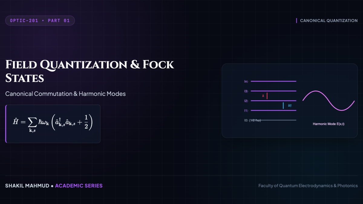
In classical electrodynamics, light is an undulating continuum of coupled electric and magnetic vector fields described by Maxwell’s partial differential equations. At the sub-microscopic quantum frontier, however, this classical continuum gives way to discrete quanta of excitation: photons. Canonical field quantization elevates classical mode amplitudes to non-commuting quantum mechanical operators, revealing the non-trivial vacuum ground state and the discrete Hilbert space of Fock number states.
1. Canonical Quantization of Free Electromagnetic Modes
Consider an empty, charge-free optical cavity of volume (V) bounded by perfectly conducting walls. Maxwell’s equations in the Coulomb gauge ((
abla cdot mathbf{A} = 0), (phi = 0)) dictate that the vector potential (mathbf{A}(mathbf{r}, t)) obeys the wave equation:
[
abla^2 mathbf{A} – rac{1}{c^2}rac{partial^2 mathbf{A}}{partial t^2} = 0
]
Expanding the classical vector potential into discrete transverse spatial Fourier modes (mathbf{u}_{mathbf{k}, s}(mathbf{r})) with wavevector (mathbf{k}) and polarization unit vector (boldsymbol{psilon}_{mathbf{k}, s}) ((s in {1, 2})):
[
mathbf{A}(mathbf{r}, t) = sum_{mathbf{k}, s} sqrt{rac{hbar}{2 psilon_0 omega_{mathbf{k}} V}} left( alpha_{mathbf{k}, s}(t) boldsymbol{psilon}_{mathbf{k}, s} e^{i mathbf{k} cdot mathbf{r}} + alpha_{mathbf{k}, s}^*(t) boldsymbol{psilon}_{mathbf{k}, s}^* e^{-i mathbf{k} cdot mathbf{r}}
ight)
]
where (omega_{mathbf{k}} = c |mathbf{k}|). To quantize the field canonically, the complex mode amplitudes (alpha_{mathbf{k}, s}) and (alpha_{mathbf{k}, s}^*) are promoted to non-Hermitian photon annihilation ((hat{a}_{mathbf{k}, s})) and creation ((hat{a}_{mathbf{k}, s}^dagger)) operators, satisfying canonical bosonic commutation relations:
[
[hat{a}_{mathbf{k}, s}, hat{a}_{mathbf{k}’, s’}^dagger] = delta_{mathbf{k}, mathbf{k}’} delta_{s, s’}, qquad [hat{a}_{mathbf{k}, s}, hat{a}_{mathbf{k}’, s’}] = [hat{a}_{mathbf{k}, s}^dagger, hat{a}_{mathbf{k}’, s’}^dagger] = 0
]
2. The Quantized Field Operators and Hamiltonian
The electric and magnetic field operators become:
[
hat{mathbf{E}}(mathbf{r}, t) = i sum_{mathbf{k}, s} sqrt{rac{hbar omega_{mathbf{k}}}{2 psilon_0 V}} boldsymbol{psilon}_{mathbf{k}, s} left( hat{a}_{mathbf{k}, s} e^{i(mathbf{k} cdot mathbf{r} – omega_{mathbf{k}} t)} – hat{a}_{mathbf{k}, s}^dagger e^{-i(mathbf{k} cdot mathbf{r} – omega_{mathbf{k}} t)}
ight)
]
[
hat{mathbf{B}}(mathbf{r}, t) = rac{i}{c} sum_{mathbf{k}, s} sqrt{rac{hbar omega_{mathbf{k}}}{2 psilon_0 V}} (hat{mathbf{k}} imes boldsymbol{psilon}_{mathbf{k}, s}) left( hat{a}_{mathbf{k}, s} e^{i(mathbf{k} cdot mathbf{r} – omega_{mathbf{k}} t)} – hat{a}_{mathbf{k}, s}^dagger e^{-i(mathbf{k} cdot mathbf{r} – omega_{mathbf{k}} t)}
ight)
]
Integrating the total field energy density over cavity volume (V) yields the multi-mode Hamiltonian operator:
[
hat{H} = rac{1}{2} int_V left( psilon_0 hat{mathbf{E}}^2 + rac{1}{mu_0}hat{mathbf{B}}^2
ight) dV = sum_{mathbf{k}, s} hbar omega_{mathbf{k}} left( hat{a}_{mathbf{k}, s}^dagger hat{a}_{mathbf{k}, s} + rac{1}{2}
ight)
]
Every electromagnetic mode behaves mathematically as an independent one-dimensional quantum harmonic oscillator of frequency (omega_{mathbf{k}}).
3. Fock Number States and Ladder Algebra
The operator (hat{n} = hat{a}^dagger hat{a}) is the Hermitian photon number operator. Its eigenstates form the discrete orthonormal Fock basis ({|n
angle}) ((n = 0, 1, 2, dots)):
[
hat{n} |n
angle = n |n
angle, qquad langle m | n
angle = delta_{mn}
]
The ladder operators step between adjacent photon number states:
[
hat{a} |n
angle = sqrt{n} |n – 1
angle, qquad hat{a}^dagger |n
angle = sqrt{n + 1} |n + 1
angle
]
An arbitrary (n)-photon Fock state is synthesized by repeatedly applying the creation operator to the vacuum ground state (|0
angle):
[
|n
angle = rac{(hat{a}^dagger)^n}{sqrt{n!}} |0
angle
]
Fock states possess strictly zero photon number uncertainty ((Delta n = sqrt{langle hat{n}^2
angle – langle hat{n}
angle^2} = 0)). By the quantum number-phase uncertainty relation ((Delta n Delta phi ge 1/2)), their optical phase is completely undefined and uniformly distributed over ([0, 2pi)).
4. The Quantum Vacuum and Zero-Point Energy
For the vacuum state (|0
angle) where no photons exist ((hat{n}|0
angle = 0)), the expectation value of the field Hamiltonian is non-zero:
[
langle 0 | hat{H} | 0
angle = sum_{mathbf{k}, s} rac{1}{2}hbar omega_{mathbf{k}}
]
Although the average electric field in vacuum vanishes ((langle 0 | hat{mathbf{E}} | 0
angle = 0)), its variance—the mean-square vacuum electric field fluctuation—is strictly positive:
[
langle 0 | hat{mathbf{E}}^2 | 0
angle = sum_{mathbf{k}} rac{hbar omega_{mathbf{k}}}{2 psilon_0 V}
e 0
]
These omnipresent zero-point quantum vacuum fluctuations are not mathematical artifacts: they drive spontaneous emission in excited atoms, induce the Lamb shift in atomic hydrogen, and generate macroscopic macroscopic attractive forces between uncharged conducting plates via the Casimir Effect.