Before 1948, the universal dogma of telecommunications engineering asserted that to transmit data faster over a noisy telephone wire or radio path, one had to inevitably accept a higher rate of errors. To eliminate errors entirely, engineers believed transmission speed had to drop toward zero. Claude Shannon utterly demolished this dogma with the Noisy-Channel Coding Theorem. He proved the existence of an intrinsic physical property of every physical channel called Channel Capacity ($C$): for any transmission rate $R < C$, there exist error-correcting codes that make the probability of error arbitrarily close to zero. Errors are not the price of speed; they are merely the consequence of unencoded transmission.
1. Discrete Memoryless Channels and The Definition of Capacity
A Discrete Memoryless Channel (DMC) consists of an input alphabet $mathcal{X}$, an output alphabet $mathcal{Y}$, and a collection of transition conditional probabilities $p(y|x)$ satisfying the memoryless condition: the output depends only on the current input, not on previous transmissions:
[
p(y_1, dots, y_n | x_1, dots, x_n) = prod_{i=1}^n p(y_i | x_i)
]
Shannon defined the Channel Capacity ($C$) as the maximum mutual information between input $X$ and output $Y$, maximized over all possible input probability distributions $p(x)$:
[
C = max_{p(x)} I(X; Y) quad text{bits per channel use}
]
Because $I(X; Y)$ is a concave function of $p(x)$ over a convex simplex, the maximum always exists and can be computed numerically using the Blahut-Arimoto algorithm.
Canonical Channel Examples:
- Binary Symmetric Channel (BSC): Bit flips occur with probability $p$. The capacity is:
[
C = 1 – H_2(p) = 1 – left( -p log_2 p – (1-p) log_2(1-p) right)
]
If $p = 0.5$ (pure noise), $C = 0$. If $p = 0.1$, $C approx 0.531$ bits/use. - Binary Erasure Channel (BEC): Bits are either received correctly or completely erased with probability $epsilon$. Its capacity is simply:
[
C = 1 – epsilon
]
2. The Noisy-Channel Coding Theorem
The crown jewel of Shannon’s 1948 paper is encapsulated in two profound statements:
- Direct (Achievability) Theorem: For any rate $R 0$, for sufficiently large block length $n$, there exists a channel code of length $n$ with $2^{nR}$ codewords such that the maximal probability of decoding error satisfies:
[
P_e^{(n)} < epsilon
] - Converse Theorem: Any code operating at transmission rate $R > C$ has a probability of error bounded away from zero; as $n to infty$, the error probability approaches $1$.
The Magic of Shannon’s Random Coding Proof
How did Shannon prove the existence of such codes when none had ever been constructed? He used a breathtaking probabilistic method: instead of designing a specific code, he considered an ensemble of random codes where each codeword bit is chosen by independent coin flips according to $p(x)$.
By analyzing joint typicality decoding—where the receiver declares that message $m$ was sent if the received output $y^n$ is jointly typical with codeword $x^n(m)$—Shannon proved that the average error probability over the entire ensemble vanishes as $n to infty$ whenever $R < C$. If the ensemble average vanishes, there must exist at least one specific code within the ensemble that performs at least as well as the average!
3. Continuous Gaussian Channels & The Shannon-Hartley Law
In physical radio channels, wirelines, and satellite links, the channel noise is continuous, additive, and Gaussian (AWGN):
[
Y_i = X_i + Z_i, quad Z_i sim mathcal{N}(0, N)
]
subject to an average transmitter power constraint $frac{1}{n}sum x_i^2 le S$.
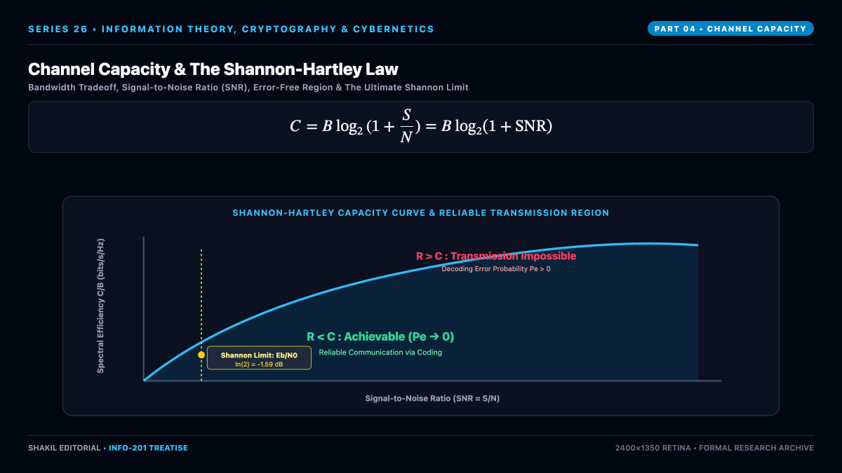
Because the Gaussian distribution uniquely maximizes differential entropy for a given variance, Shannon proved that the optimal input distribution is also Gaussian ($X sim mathcal{N}(0, S)$). Extending this to a continuous-time channel with physical bandwidth $B$ (in Hertz) sampled at the Nyquist rate $2B$ samples/second yields the immortal Shannon-Hartley Theorem:
[
C = B log_2 left( 1 + frac{S}{N} right) = B log_2(1 + text{SNR}) quad text{bits/second}
]
The Shannon-Hartley formula dictates how bandwidth $B$ and signal power $S$ can be traded off:
- Bandwidth-Limited Regime ($text{SNR} gg 1$): Capacity grows logarithmically with power, but linearly with bandwidth $C approx B log_2(text{SNR})$.
- Power-Limited Regime ($text{SNR} ll 1$): In deep space communications, bandwidth is effectively infinite ($B to infty$). Using $ln(1 + x) approx x$ as $x to 0$:
[
C_infty = lim_{B to infty} B log_2left(1 + frac{S}{N_0 B}right) = frac{S}{N_0 ln 2} approx 1.442 frac{S}{N_0} text{ bits/s}
]
Expressing this in terms of the energy per bit $E_b = S / C$, we derive the Ultimate Shannon Limit:
[
frac{E_b}{N_0} ge ln 2 approx 0.693 iff frac{E_b}{N_0} ge -1.59 text{ dB}
]
No communication system in the universe, regardless of modulation, coding, or antenna architecture, can achieve error-free communication if $E_b / N_0 < -1.59 text{ dB}$. Modern 5G and satellite codes operate within $0.1 text{ dB}$ of this cosmic frontier.