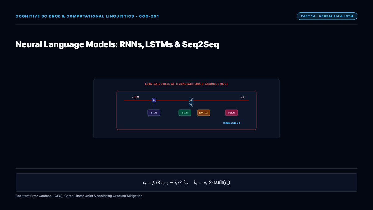
While statistical n-gram models are intrinsically hamstrung by Markov context cutoffs, Recurrent Neural Networks (RNNs) theoretically process arbitrary-length historical contexts by maintaining a continuous recurrent hidden state. Overcoming the catastrophic vanishing gradient problem via gated memory units, LSTMs and Seq2Seq models sparked the modern era of deep learning in NLP.
1. The Vanilla Recurrent Neural Network (Elman RNN)
In a standard Recurrent Neural Network (Elman, 1990), word tokens (x_t in mathbb{R}^d) are processed sequentially. At each time step (t), the network updates its internal continuous memory (hidden state (mathbf{h}_t in mathbb{R}^h)) by linearly combining the current input embedding with the previous hidden state (mathbf{h}_{t-1}):
[
mathbf{h}_t = anhleft( mathbf{W}_{hh} mathbf{h}_{t-1} + mathbf{W}_{xh} mathbf{x}_t + mathbf{b}_h
ight)
]
The conditional probability distribution over the vocabulary is generated via affine transformation and softmax:
[
hat{mathbf{y}}_t = P(w_{t+1} mid w_1 dots w_t) = ext{softmax}left( mathbf{W}_{hy} mathbf{h}_t + mathbf{b}_y
ight)
]
2. Backpropagation Through Time (BPTT) and The Vanishing Gradient Catastrophe
Training an RNN involves unrolling the network over (T) time steps and propagating loss gradients backward via Backpropagation Through Time (BPTT). The gradient of the loss at step (T) with respect to the hidden state at an earlier step (t) involves a Jacobian product chain rule:
[
rac{partial mathcal{L}_T}{partial mathbf{h}_t} = rac{partial mathcal{L}_T}{partial mathbf{h}_T} prod_{k=t+1}^T rac{partial mathbf{h}_k}{partial mathbf{h}_{k-1}} = rac{partial mathcal{L}_T}{partial mathbf{h}_T} prod_{k=t+1}^T ext{diag}left( 1 – anh^2(mathbf{a}_k)
ight) mathbf{W}_{hh}^ op
]
Bengio et al. (1994) proved that as the temporal distance (T – t) increases, this repeated matrix multiplication undergoes an exponential bifurcation:
- If the spectral radius (largest eigenvalue) (
ho(mathbf{W}_{hh}) > 1), gradients diverge exponentially to infinity (( o infty)), causing numerical exploding gradients. - If (
ho(mathbf{W}_{hh}) < 1) or because (|1 – anh^2(x)| le 1), gradients contract exponentially toward zero (( o 0)), triggering the vanishing gradient catastrophe.
Vanishing gradients render vanilla RNNs incapable of learning grammatical dependencies spanning more than (5 – 10) words (such as long-distance subject-verb agreement across embedded clauses).
3. Long Short-Term Memory (LSTM) Architecture
In 1997, Sepp Hochreiter and Jürgen Schmidhuber resolved the vanishing gradient catastrophe by introducing the Long Short-Term Memory (LSTM) network. The definitive breakthrough was the introduction of an internal cell state (mathbf{c}_t) acting as a linear constant error carousel (CEC).
Information flow into and out of (mathbf{c}_t) is regulated by three multiplicative sigmoid gating units ((sigma(z) in [0, 1])):
[
begin{aligned}
ext{Forget Gate: } & mathbf{f}_t = sigmaleft( mathbf{W}_f [mathbf{h}_{t-1}, mathbf{x}_t] + mathbf{b}_f
ight)
ext{Input Gate: } & mathbf{i}_t = sigmaleft( mathbf{W}_i [mathbf{h}_{t-1}, mathbf{x}_t] + mathbf{b}_i
ight)
ext{Candidate State: } & ilde{mathbf{c}}_t = anhleft( mathbf{W}_c [mathbf{h}_{t-1}, mathbf{x}_t] + mathbf{b}_c
ight)
ext{Cell State Update: } & mathbf{c}_t = mathbf{f}_t odot mathbf{c}_{t-1} + mathbf{i}_t odot ilde{mathbf{c}}_t
ext{Output Gate: } & mathbf{o}_t = sigmaleft( mathbf{W}_o [mathbf{h}_{t-1}, mathbf{x}_t] + mathbf{b}_o
ight)
ext{Hidden State: } & mathbf{h}_t = mathbf{o}_t odot anh(mathbf{c}_t)
nd{aligned}
]
Crucially, because the cell update (mathbf{c}_t = mathbf{f}_t odot mathbf{c}_{t-1} + dots) is strictly additive rather than multiplicative, the gradient (rac{partial mathbf{c}_t}{partial mathbf{c}_{t-1}} = mathbf{f}_t). If the forget gate is saturated at (1), gradients propagate backward across hundreds of time steps with zero exponential attenuation, preserving long-range syntactic agreement.
4. The Sequence-to-Sequence (Seq2Seq) Paradigm
In 2014, Ilya Sutskever et al. (Google) and Kyunghyun Cho et al. introduced the Seq2Seq encoder-decoder architecture, revolutionizing neural machine translation.
- Encoder: An LSTM reads input sequence ((x_1, dots, x_{T_x})) word-by-word, compressing its entire semantic meaning into a fixed-dimensional vector: the final hidden state (mathbf{h}_{T_x}).
- Decoder: A second LSTM takes this thought vector as its initial hidden state and auto-regressively generates target words ((y_1, y_2, dots)) one token at a time until emitting an end-of-sequence token
<EOS>.
Seq2Seq established the universal paradigm for machine translation, summarization, and dialogue generation, paving the direct path toward attention mechanisms and the Transformer.