Before the dominance of deep neural networks, statistical language modeling formed the computational bedrock of speech recognition, machine translation, and predictive text. By modeling the probability distribution over word sequences using Markovian assumptions and sophisticated backoff smoothing, statistical n-grams quantified the structural predictability of natural language.
1. The Language Modeling Objective and The Chain Rule
A probabilistic language model assigns a joint probability (P(W)) to any arbitrary sequence of (N) words (W = (w_1, w_2, dots, w_N)). Invoking the classical probability chain rule without loss of generality:
[
P(w_1, w_2, dots, w_N) = prod_{k=1}^N P(w_k mid w_1, w_2, dots, w_{k-1})
]
Evaluating the conditional probability (P(w_k mid w_1^{k-1})) directly is computationally impossible because natural language history strings grow without bound, generating infinite conditioning contexts that can never be observed in finite training corpora.
2. The Markov Assumption and Maximum Likelihood Estimation
To make probability estimation tractable, the Markov assumption posits that the probability of the upcoming word depends only on the immediately preceding (n-1) words:
[
P(w_k mid w_1^{k-1}) approx P(w_k mid w_{k-n+1}^{k-1})
]
For an (n)-gram model:
- Unigram ((n=1)): (P(w_k)) (assumes independent identical distribution; word bag).
- Bigram ((n=2)): (P(w_k mid w_{k-1})) (first-order Markov chain).
- Trigram ((n=3)): (P(w_k mid w_{k-2}, w_{k-1})) (second-order Markov chain).
Under Maximum Likelihood Estimation (MLE), conditional probabilities are computed simply by normalizing raw frequency counts extracted from a text corpus:
[
P_{ ext{MLE}}(w_k mid w_{k-1}) = rac{C(w_{k-1}, w_k)}{sum_w C(w_{k-1}, w)} = rac{C(w_{k-1}, w_k)}{C(w_{k-1})}
]
3. The Zero-Probability Sparsity Problem and Perplexity
The fatal flaw of raw MLE is data sparsity. Because natural language vocabulary size (|V|) is large ((|V| sim 10^5 – 10^6)), the number of possible trigrams scales as (|V|^3 sim 10^{15}). In any finite corpus, the vast majority of valid, grammatical n-grams are never observed ((C = 0)).
If an unseen test sentence contains even a single novel bigram with count zero, the product of probabilities collapses to zero:
[
P_{ ext{MLE}}( ext{Sentence}) = 0
]
Language model performance is quantified across held-out test data by Perplexity (PPL), defined as the inverse geometric mean probability of the token sequence:
[
ext{PPL}(W) = P(w_1, dots, w_N)^{-1/N} = xpleft( -rac{1}{N} sum_{k=1}^N ln P(w_k mid w_1^{k-1})
ight)
]
Lower perplexity indicates higher predictive accuracy. If (P = 0), perplexity diverges to infinity (( ext{PPL} o infty)), rendering raw MLE unusable.
4. Modified Kneser-Ney Smoothing: State of the Art
To prevent probability collapse, probability mass must be shaved off frequently observed n-grams and redistributed (smoothed) onto unseen events. Early techniques—such as Laplace add-one smoothing or Good-Turing frequency discounting—proved crude and biased.
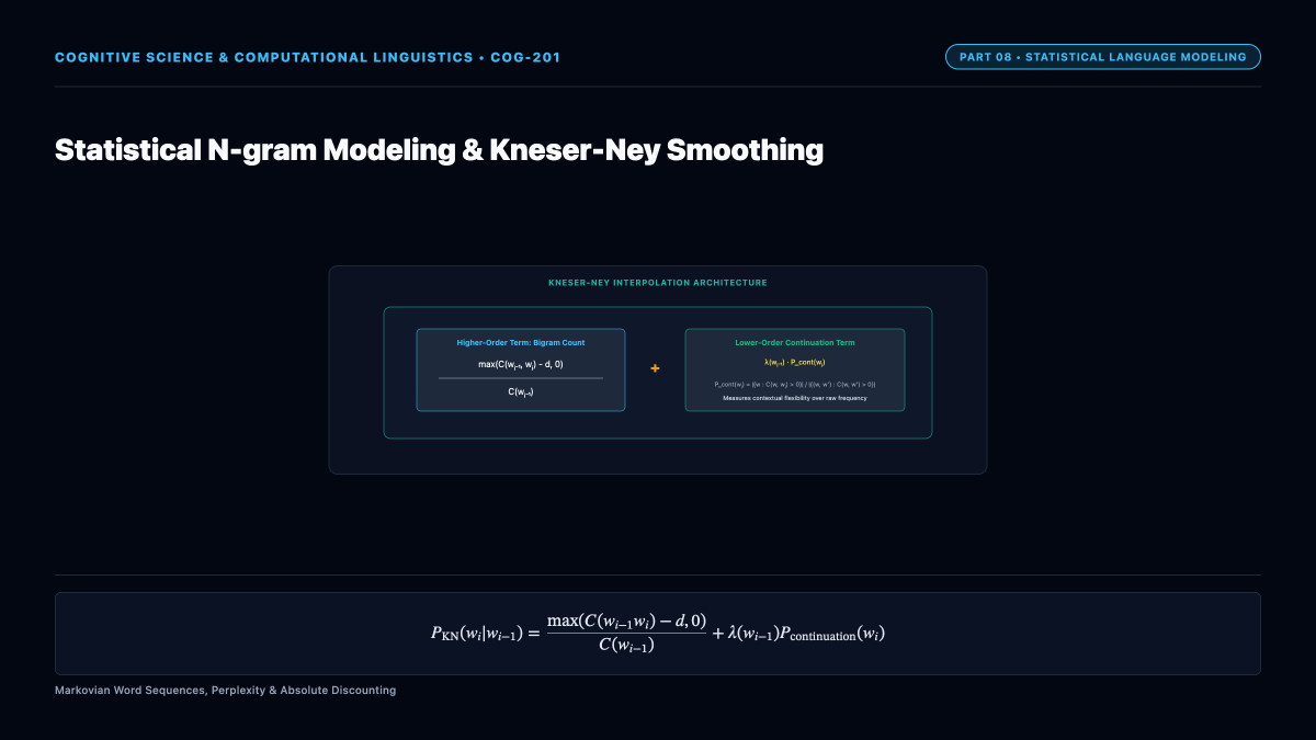
In 1995, Reinhard Kneser and Hermann Ney formulated Kneser-Ney smoothing, which remains the mathematical gold standard of statistical n-gram estimation. Kneser-Ney incorporates two foundational innovations:
1. Absolute Discounting
Empirical analysis of text shows that high-frequency n-grams consistently lose an approximately constant absolute probability mass (d in (0, 1)) (typically (d approx 0.75)) compared to their MLE counts:
[
P(w_i mid w_{i-1}) = rac{max(C(w_{i-1}, w_i) – d, 0)}{C(w_{i-1})} + lambda(w_{i-1}) P_{ ext{lower}}(w_i)
]
where the normalization coefficient (lambda(w_{i-1})) ensures the distribution sums strictly to unity:
[
lambda(w_{i-1}) = rac{d}{C(w_{i-1})} cdot left| { w : C(w_{i-1}, w) > 0 }
ight|
]
2. Continuation Probability
The revolutionary core of Kneser-Ney is its formulation of the lower-order backoff distribution. Consider the unigram “San Francisco”. The word “Francisco” has very high unigram frequency in general text. Under naive unigram backoff, if an unseen context occurs (e.g., “I want to read a novel by Francisco”), naive unigram backoff would assign high probability to “Francisco”.
Kneser-Ney recognizes that “Francisco” occurs almost exclusively after the single word “San”. Instead of raw unigram frequency, Kneser-Ney defines the lower-order term by its continuation probability—counting how many distinct preceding words the target word can follow:
[
P_{ ext{continuation}}(w) = rac{left| { w’ : C(w’, w) > 0 }
ight|}{sum_{w”} left| { w’ : C(w’, w”) > 0 }
ight|}
]
Words with high continuation probability are contextually versatile (like “read”, “time”, or “thing”), making them far more plausible as completions for novel contexts. In Modified Kneser-Ney (Chen and Goodman, 1996), three distinct discounts (d_1, d_2, d_{3+}) are optimized for counts of 1, 2, and 3+, achieving unmatched statistical predictive accuracy.