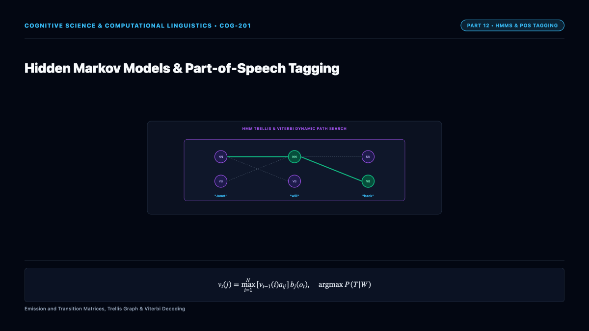
Part-of-Speech (POS) tagging—annotating every word in a running text with its correct grammatical category (Noun, Verb, Adjective, Preposition)—is the foundational pre-processing stage of natural language processing. In the stochastic framework, POS tagging is formalized as an optimal state inference problem over Hidden Markov Models (HMMs).
1. The Sequence Labeling Problem and Syntactic Ambiguity
Given an observed sequence of (T) surface words (W = (w_1, w_2, dots, w_T)), the goal of POS tagging is to select the most probable sequence of grammatical tags (hat{T} = (t_1, t_2, dots, t_T)) from a tagset (such as the 45-tag Penn Treebank set). Many common words are wildly ambiguous across categories:
- “book”: Noun (“read a book”) vs Verb (“book a flight”).
- “back”: Noun, Verb, Adjective, or Adverb.
- “that”: Determiner, Complementizer, Relative Pronoun, or Adverb.
Invoking Bayes’ theorem, the optimal sequence maximizes the joint posterior probability:
[
hat{T} = argmax_T P(T mid W) = argmax_T rac{P(W mid T) P(T)}{P(W)} = argmax_T P(W mid T) P(T)
]
2. The Hidden Markov Model (HMM) Mathematical Formulation
A Hidden Markov Model is a doubly embedded stochastic process where the underlying state sequence (T = (t_1, dots, t_T)) is an unobservable (hidden) Markov chain, and the surface observation sequence (W = (w_1, dots, w_T)) is probabilistic emissions from those states. An HMM is specified by the 5-tuple:
[
lambda = langle S, V, A, B, pi
angle
]
where:
- (S = { s_1, s_2, dots, s_N }) is the set of (N) hidden states (POS tags).
- (V = { v_1, v_2, dots, v_M }) is the finite vocabulary of (M) observable words.
- (A = { a_{ij} }) is the state transition probability matrix, satisfying the first-order Markov assumption:
[
a_{ij} = P(t_k = s_j mid t_{k-1} = s_i)
] - (B = { b_j(w_k) }) is the emission probability matrix, satisfying the output independence assumption:
[
b_j(w_k) = P(w_k mid t_k = s_j)
] - (pi = { pi_i }) is the initial state distribution: (pi_i = P(t_1 = s_i)).
Under these dual independence assumptions, the joint probability of a sequence of words and tags simplifies into a tractable product:
[
P(W, T) = prod_{k=1}^T P(t_k mid t_{k-1}) P(w_k mid t_k) = prod_{k=1}^T a_{t_{k-1}, t_k} b_{t_k}(w_k)
]
3. Maximum Likelihood Parameter Estimation from Corpora
Given a supervised training corpus (such as the Penn Treebank), the transition and emission matrices are estimated via smoothed Maximum Likelihood counts:
[
a_{ij} = rac{C(t_i, t_j) + psilon}{C(t_i) + psilon N}, quad b_j(w_k) = rac{C(t_j, w_k) + psilon}{C(t_j) + psilon M}
]
4. The Viterbi Dynamic Programming Decoding Algorithm
For a sentence of length (T) and tagset size (N), there exist (N^T) possible candidate tag sequences (for (N=45, T=20), (N^T approx 10^{33})). Evaluating each path individually is computationally impossible.
The Viterbi algorithm solves this globally optimal decoding problem in polynomial time (mathcal{O}(T cdot N^2)) by applying dynamic programming across a trellis graph.
The Viterbi Trellis Formulation:
Define (v_t(j)) as the maximum joint probability of the most likely hidden tag sequence ending in state (s_j) at time step (t), having observed the initial word prefix (w_1 dots w_t):
[
v_t(j) = max_{t_1, dots, t_{t-1}} P(w_1 dots w_t, t_1 dots t_{t-1}, t_t = s_j)
]
Viterbi Algorithmic Steps:
- Initialization ((t = 1)):
[
v_1(j) = pi_j b_j(w_1), quad ext{backpointer } bp_1(j) = 0, quad 1 le j le N
] - Induction ((t = 2) to (T)):
[
v_t(j) = max_{i=1}^N left[ v_{t-1}(i) a_{ij}
ight] b_j(w_t), quad 1 le j le N
]
[
bp_t(j) = argmax_{i=1}^N left[ v_{t-1}(i) a_{ij}
ight]
] - Termination:
[
P^* = max_{i=1}^N v_T(i), quad hat{t}_T = argmax_{i=1}^N v_T(i)
] - Backtracking:
[
hat{t}_{t-1} = bp_t(hat{t}_t), quad t = T, T-1, dots, 2
]
The Viterbi algorithm guarantees identifying the mathematically optimal global sequence of POS tags, achieving tag accuracies above (97%) and providing the foundational architecture for acoustic speech recognition and named entity recognition.