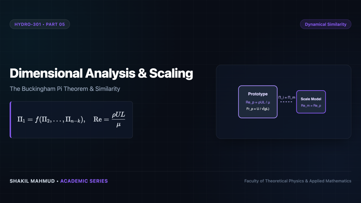
Experimental and computational fluid dynamics face a daunting reality: testing full-scale ocean vessels, transcontinental airliners, or atmospheric circulation patterns directly is often physically or economically impossible. Dimensional analysis bridges this gap by transforming complex multivariable physical equations into universal dimensionless groups, ensuring complete physical similitude between scaled laboratory models and full-sized prototypes.
1. The Foundation of Physical Dimensions and Units
In classical fluid mechanics, all physical quantities can be expressed in terms of four fundamental base dimensions: Mass (( ext{M})), Length (( ext{L})), Time (( ext{T})), and Temperature ((Theta)). The principle of dimensional homogeneity demands that any physically valid equation must balance fundamental dimensions across every additive term.
2. The Buckingham (pi) Theorem
Formulated by Edgar Buckingham in 1914, the theorem provides a rigorous algebraic algorithm for determining the minimum number of independent dimensionless parameters required to describe a physical phenomenon:
Theorem: If a physical relation involves (n) dimensional physical variables:
[
f(q_1, q_2, dots, q_n) = 0
]
and these variables span (k) fundamental physical dimensions (equal to the rank of the dimensional matrix), then the relation can be reformulated entirely in terms of (p = n – k) independent dimensionless groups ((Pi_1, Pi_2, dots, Pi_p)):
[
Phi(Pi_1, Pi_2, dots, Pi_{n-k}) = 0
]
The Method of Repeating Variables
- List the (n) relevant physical variables (e.g., drag force (F_D), velocity (U), linear dimension (L), density (
ho), viscosity (mu), speed of sound (a)). - Construct the (k imes n) dimensional matrix and determine its rank (k) (typically (k=3) for ( ext{M, L, T})).
- Select (k) repeating variables that do not themselves form a dimensionless group and collectively span all (k) dimensions (e.g., (
ho, U, L)). - Form each dimensionless (Pi)-group by multiplying a non-repeating variable with the repeating variables raised to unknown exponents and solving for dimensional neutrality:
[
Pi_i = q_i cdot
ho^a U^b L^c implies [Pi_i] = ext{M}^0 ext{L}^0 ext{T}^0
]
3. Canonical Dimensionless Numbers in Fluid Mechanics
| Dimensionless Group | Definition | Physical Ratio | Dominant Regime |
|---|---|---|---|
| Reynolds Number ((mathrm{Re})) | (rac{ ho U L}{mu} = rac{U L}{ u}) |
Inertial Forces / Viscous Shear Forces | Laminar-to-turbulent transition |
| Mach Number ((mathrm{Ma})) | (rac{U}{a} = rac{U}{sqrt{gamma R T}}) | Flow Speed / Speed of Sound | Compressibility effects ((mathrm{Ma} > 0.3)) |
| Froude Number ((mathrm{Fr})) | (rac{U}{sqrt{g L}}) | Inertial Forces / Gravitational Forces | Free-surface waves, ship hydrodynamics |
| Knudsen Number ((mathrm{Kn})) | (rac{lambda}{L}) | Molecular Mean Free Path / Macro Scale | Continuum breakdown, rarefied gas dynamics |
| Weber Number ((mathrm{We})) | (rac{ ho U^2 L}{sigma}) |
Inertial Forces / Surface Tension Forces | Droplet breakup, bubble dynamics |
4. The Doctrine of Dynamical Similitude
To ensure that a scale model tested in a wind tunnel or water flume faithfully predicts the aerodynamic behavior of a full-scale aircraft or submarine, three hierarchical tiers of similarity must be satisfied simultaneously:
- Geometric Similitude: The model and prototype must possess identical spatial proportions, with all linear dimensions scaled by a uniform factor (lambda_L = L_m / L_p).
- Kinematic Similitude: Velocity vectors at homologous spatial points must point in identical directions and scale by a constant velocity ratio (lambda_U = U_m / U_p), ensuring identical streamline topographies.
- Dynamic Similitude: All force ratios must be identical at homologous points, requiring exact equality of all governing dimensionless numbers:
[
mathrm{Re}_m = mathrm{Re}_p, quad mathrm{Ma}_m = mathrm{Ma}_p, quad mathrm{Fr}_m = mathrm{Fr}_p
]
When multiple dimensionless numbers conflict (e.g., simultaneously matching (mathrm{Re}) and (mathrm{Fr}) in naval ship testing requires fluids with unattainable kinematic viscosities (
u_m =
u_p lambda_L^{3/2})), engineers employ William Froude’s superposition hypothesis: separating total hydrodynamic resistance into wave-making resistance (governed strictly by (mathrm{Fr})) and skin-friction drag (governed by (mathrm{Re})).