Turbulence is ubiquitous yet remains the last great unsolved classical physics puzzle. In the famous words attributed to Werner Heisenberg: “When I meet God, I am going to ask him two questions: Why relativity? And why turbulence? I really believe he will have an answer for the first.” The transition to turbulence transforms orderly deterministic trajectories into a high-dimensional, spatiotemporally chaotic attractor.
1. The Path of Natural Transition
In low-disturbance environments, the route from a laminar boundary layer to fully developed turbulence proceeds through four well-defined chronological stages:
- Primary Instability (Tollmien-Schlichting Waves): Weak environmental acoustic or freestream disturbances penetrate the boundary layer, exciting 2D viscous instability waves predicted by the Orr-Sommerfeld equation.
- Secondary Instability (3D Breakdown): The 2D Tollmien-Schlichting waves attain finite amplitudes, warping into 3D staggered (Lambda)-vortices via Craik or Herbert resonant triad interactions.
- Turbulent Spots (Emmons Spots): Hairpin vortices stretch violently, undergoing local viscous breakdown that nucleates isolated, arrow-shaped islands of high-frequency turbulence called Emmons spots.
- Full Coalescence: Turbulent spots grow at a half-angle of (sim 10^circ) as they convect downstream, coalescing into an unbroken, fully turbulent boundary layer.
Alternatively, in environments with intense freestream turbulence ((>1%)) or surface roughness, the linear wave stage is bypassed entirely—a phenomenon known as bypass transition driven by transient growth of streamwise streaks.
2. Reynolds Decomposition and Averaging
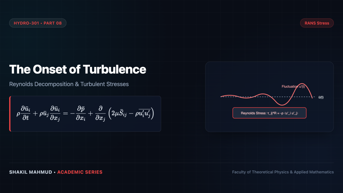
To analyze the chaotic velocity and pressure fields, Osborne Reynolds (1895) introduced statistical decomposition: partitioning every instantaneous flow variable (phi(mathbf{x}, t)) into an ensemble (or temporal) mean (bar{phi}(mathbf{x})) and a zero-mean turbulent fluctuation (phi'(mathbf{x}, t)):
[
u_i(mathbf{x}, t) = bar{u}_i(mathbf{x}) + u’_i(mathbf{x}, t), quad p(mathbf{x}, t) = bar{p}(mathbf{x}) + p'(mathbf{x}, t)
]
where by definition, the average of the fluctuation is strictly zero: (overline{u’_i} = 0), but the average of non-linear products of fluctuations is non-zero: (overline{u’_i u’_j}
e 0).
3. The Reynolds-Averaged Navier-Stokes (RANS) Equations
Applying the Reynolds averaging operator to the incompressible Navier-Stokes momentum equation:
[
overline{ rac{partial u_i}{partial t} + rac{partial(u_i u_j)}{partial x_j} } = overline{ -rac{1}{
ho}rac{partial p}{partial x_i} +
u rac{partial^2 u_i}{partial x_j partial x_j} }
]
Because (overline{u_i u_j} = bar{u}_i bar{u}_j + overline{u’_i u’_j}), the non-linear convective acceleration splits, yielding the RANS equations:
[
ho left( rac{partial bar{u}_i}{partial t} + bar{u}_j rac{partial bar{u}_i}{partial x_j}
ight) = -rac{partial bar{p}}{partial x_i} + rac{partial}{partial x_j} left( 2mu bar{S}_{ij} –
ho overline{u’_i u’_j}
ight)
]
where (bar{S}_{ij} = rac{1}{2}(partial bar{u}_i / partial x_j + partial bar{u}_j / partial x_i)) is the mean rate-of-strain tensor.
4. The Reynolds Stress Tensor and The Closure Problem
The term (-
ho overline{u’_i u’_j}) is the symmetric second-rank Reynolds stress tensor (boldsymbol{ au}^R):
[
boldsymbol{ au}^R = –
ho begin{bmatrix}
overline{u’^2} & overline{u’v’} & overline{u’w’}
overline{u’v’} & overline{v’^2} & overline{v’w’}
overline{u’w’} & overline{v’w’} & overline{w’^2}
nd{bmatrix}
]
Physically, the diagonal components ((-
ho overline{u’^2}), etc.) represent turbulent normal stresses, while the off-diagonal components ((-
ho overline{u’v’})) represent turbulent shear stresses arising from cross-stream convective momentum transport by fluctuating eddies.
The Fundamental Closure Problem
Averaging a non-linear differential equation introduces higher-order statistical moments. In RANS, we have 4 governing equations (1 continuity + 3 momentum), but 10 unknowns: 1 mean pressure (bar{p}), 3 mean velocity components (bar{u}_i), and 6 independent components of the symmetric Reynolds stress tensor (boldsymbol{ au}^R).
Attempting to derive exact transport equations for (overline{u’_i u’_j}) inevitably introduces third-order triple correlations (overline{u’_i u’_j u’_k}) and pressure-strain rate correlations. This fundamental mismatch—requiring more equations than are available—is the notorious closure problem of turbulence, necessitating semi-empirical turbulence modeling (e.g., Boussinesq eddy viscosity, (k ext{-}psilon), (k ext{-}omega) SST).