Vorticity is the sinew and muscle of fluid motion. Described by Horace Lamb as the intrinsic rotating essence of real flows, vorticity quantifies the local angular rotation of microscopic fluid elements. Its transport, stretching, and dissipation govern phenomena ranging from wingtip trailing vortices and smoke rings to atmospheric cyclones and turbulent cascades.
1. Kinematics of Vorticity
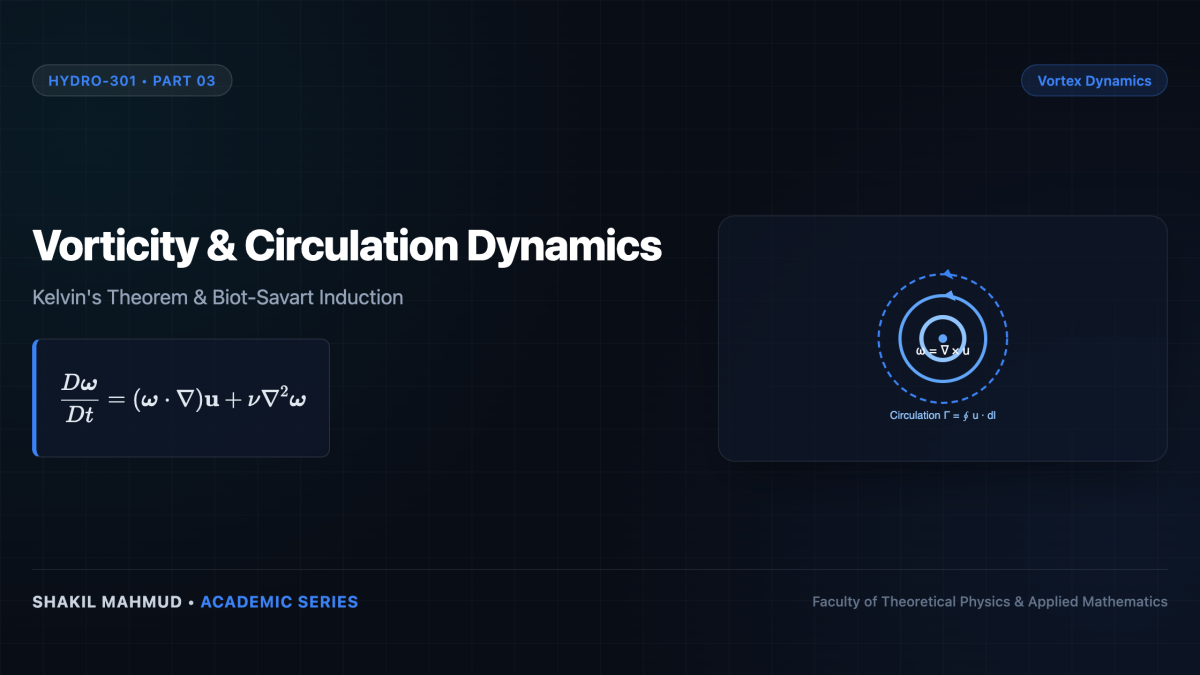
The vorticity vector (boldsymbol{omega}) is defined mathematically as the curl of the Eulerian velocity field (mathbf{u}):
[
boldsymbol{omega} quiv
abla imes mathbf{u}
]
Vorticity is intrinsically solenoidal by vector calculus identity: (
abla cdot boldsymbol{omega} =
abla cdot (
abla imes mathbf{u}) quiv 0). This implies that vortex lines can never end abruptly within a fluid; they must either form closed loops (e.g., vortex rings), extend to boundaries, or terminate at infinity.
The microscopic physical meaning of (boldsymbol{omega}) is direct: it represents twice the instantaneous local angular velocity (boldsymbol{Omega}_f) of a fluid element: (boldsymbol{omega} = 2boldsymbol{Omega}_f).
2. The Vorticity Transport Equation
Taking the mathematical curl of the Navier-Stokes momentum equation under constant viscosity eliminates the isotropic pressure gradient ((
abla imes
abla p = mathbf{0})), yielding the fundamental vorticity transport equation:
[
rac{partial boldsymbol{omega}}{partial t} + (mathbf{u} cdot
abla)boldsymbol{omega} = (boldsymbol{omega} cdot
abla)mathbf{u} +
u
abla^2 boldsymbol{omega} + rac{1}{
ho^2}(
abla
ho imes
abla p)
]
Expressed via the material derivative (Dboldsymbol{omega}/Dt):
[
rac{Dboldsymbol{omega}}{Dt} = underbrace{(boldsymbol{omega} cdot
abla)mathbf{u}}_{ ext{Vortex Stretching & Tilting}} + underbrace{
u
abla^2 boldsymbol{omega}}_{ ext{Viscous Diffusion}} + underbrace{rac{1}{
ho^2}(
abla
ho imes
abla p)}_{ ext{Baroclinic Torque}}
]
Vortex Stretching: The Engine of 3D Turbulence
The term ((boldsymbol{omega} cdot
abla)mathbf{u}) represents vortex stretching and tilting. If a vortex filament aligned along the (z)-axis experiences a velocity gradient (partial u_z / partial z > 0), the filament is elongated along its axis. By mass conservation, its cross-sectional area contracts. To conserve angular momentum, its spin rate accelerates dramatically. Crucially, vortex stretching is identically zero in two-dimensional flows (where (boldsymbol{omega}) is strictly perpendicular to the flow plane), explaining why 2D turbulence displays an inverse energy cascade while 3D turbulence drives relentless forward energy cascades down to dissipative scales.
Baroclinic Torque
When surfaces of constant density (isopycnals) are misaligned with surfaces of constant pressure (isobars), the cross-product (
abla
ho imes
abla p
e mathbf{0}). This generates baroclinic vorticity, driving sea breezes, atmospheric frontal weather systems, and oceanic gyres.
3. Kelvin’s Circulation Theorem and Helmholtz Laws
Circulation ((Gamma)) is the line integral of velocity around a closed material contour (C):
[
Gamma = oint_C mathbf{u} cdot dmathbf{l} = iint_S (
abla imes mathbf{u}) cdot dmathbf{A} = iint_S boldsymbol{omega} cdot dmathbf{A}
]
Kelvin’s Circulation Theorem establishes that in an inviscid ((
u = 0)), barotropic ((
ho =
ho(p))) fluid with conservative body forces, circulation around a material contour moving with the fluid is strictly conserved:
[
rac{DGamma}{Dt} = 0
]
This underpins Helmholtz’s Vortex Theorems:
- Vortex lines move as material lines frozen into the fluid.
- The circulation (vortex strength) along any cross-section of a vortex tube is constant along its entire length.
- The vortex strength remains invariant over time under inviscid motion.
4. The Biot-Savart Law for Induced Velocity
In incompressible, unbounded flows, the velocity field (mathbf{u}(mathbf{x})) can be reconstructed entirely from the spatial distribution of vorticity (boldsymbol{omega}(mathbf{x}’)) using the hydrodynamic analog of the electromagnetic Biot-Savart Law:
[
mathbf{u}(mathbf{x}) = -rac{1}{4pi} iiint_{mathbb{R}^3} rac{(mathbf{x} – mathbf{x}’) imes boldsymbol{omega}(mathbf{x}’)}{|mathbf{x} – mathbf{x}’|^3} , dV’
]
For an isolated straight line vortex filament of circulation (Gamma), integration yields the classic circumferential induced velocity field: (u_ heta(r) = rac{Gamma}{2pi r}).