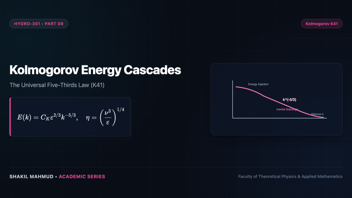
Lewis Fry Richardson famously summarized turbulent dynamics in verse: “Big whirls have little whirls that feed on their velocity, and little whirls have lesser whirls and so on to viscosity.” In 1941, the monumental Soviet mathematician Andrey Kolmogorov formalized this poetic intuition into a profound statistical theory (K41), deriving the universal five-thirds power law governing turbulent kinetic energy.
1. The Richardson Energy Cascade
In high-Reynolds-number turbulent flows, kinetic energy is injected at macroscopic integral length scales (L) by mean shear or boundary forcing. These massive primary eddies (wavenumber (k sim 1/L)) are dynamically unstable; they undergo vortex stretching and break down into progressively smaller daughter eddies.
Because molecular viscosity is utterly negligible at these large and intermediate scales, kinetic energy is transferred conservatively downward through the scales without dissipation. The cascade proceeds step by step until eddies become so microscopic that local velocity gradients become immense, allowing molecular viscosity to directly dissipate kinetic energy into thermodynamic heat.
2. Kolmogorov’s 1941 Hypotheses (K41)
Kolmogorov posited three foundational physical hypotheses for statistically stationary, homogeneous, and isotropic turbulence at Reynolds numbers approaching infinity ((mathrm{Re} o infty)):
Hypothesis 1: Local Isotropy
At sufficiently high Reynolds numbers, the small-scale turbulent motions ((r ll L)) lose all directional memory of the large-scale anisotropic boundary conditions and mean shear, becoming statistically homogeneous and isotropic.
Hypothesis 2: First Similarity Hypothesis
The statistical state of small-scale eddies is uniquely and completely determined by two physical parameters: the kinematic viscosity (
u) and the mean rate of turbulent kinetic energy dissipation per unit mass (arepsilon) (([arepsilon] = ext{m}^2/ ext{s}^3 = ext{W/kg})).
From dimensional analysis, this yields the universal Kolmogorov microscale:
[
ext{Length Scale: } ta = left( rac{
u^3}{arepsilon}
ight)^{1/4}, quad ext{Time Scale: } au_ta = left( rac{
u}{arepsilon}
ight)^{1/2}, quad ext{Velocity Scale: } u_ta = (
u arepsilon)^{1/4}
]
At scale (ta), the local eddy Reynolds number is identically unity: (mathrm{Re}_ta = u_ta ta /
u quiv 1), marking the exact frontier where viscous dissipation arrests inertial cascading.
Hypothesis 3: Second Similarity Hypothesis (The Inertial Subrange)
In the intermediate range of scales (ta ll r ll L)—designated the inertial subrange—viscous effects are negligible ((
u) drops out), and large-scale geometry is forgotten. Therefore, the statistics of eddies in this range depend strictly and solely upon (arepsilon).
3. Derivation of the Universal -5/3 Energy Spectrum
Let (E(k)) denote the three-dimensional turbulent kinetic energy spectrum, such that the total turbulent kinetic energy (k_t) is the integral over all wavenumbers:
[
k_t = int_0^infty E(k) , dk, quad [E(k)] = rac{ ext{m}^3}{ ext{s}^2}
]
In the inertial subrange, (E(k)) can depend only on the wavenumber (k) (([k] = ext{m}^{-1})) and the energy dissipation rate (arepsilon) (([arepsilon] = ext{m}^2/ ext{s}^3)). Formulating a dimensional power law:
[
E(k) = C_K , arepsilon^a k^b
]
Equating dimensions: ( ext{L}^3 ext{T}^{-2} = ( ext{L}^2 ext{T}^{-3})^a ( ext{L}^{-1})^b = ext{L}^{2a – b} ext{T}^{-3a}). Solving the linear algebraic system:
[
-3a = -2 implies a = rac{2}{3}, quad 2left(rac{2}{3}
ight) – b = 3 implies b = -rac{5}{3}
]
This yields the celebrated Kolmogorov Five-Thirds Law:
[
E(k) = C_K , arepsilon^{2/3} k^{-5/3}
]
where (C_K approx 1.5) is the universal Kolmogorov constant, validated experimentally across wind tunnels, atmospheric boundary layers, oceanic thermoclines, and interstellar molecular clouds.
4. The Range of Scales and Degrees of Freedom
Because (arepsilon sim U^3 / L), the ratio of the macroscopic integral scale (L) to the microscopic Kolmogorov dissipation scale (ta) scales algebraically with the Reynolds number:
[
rac{L}{ta} sim left( rac{U L}{
u}
ight)^{3/4} = mathrm{Re}^{3/4}
]
In three-dimensional turbulence, the number of spatial degrees of freedom (N_{ ext{DOF}}) required to resolve every eddy down to (ta) in a Direct Numerical Simulation (DNS) scales as:
[
N_{ ext{DOF}} sim left( rac{L}{ta}
ight)^3 sim mathrm{Re}^{9/4}
]
For an airliner cruising at (mathrm{Re} approx 10^8), (N_{ ext{DOF}} sim 10^{18}) grid points—requiring exaflop supercomputers that place full-airplane DNS beyond contemporary reach, highlighting why turbulence modeling remains vital.