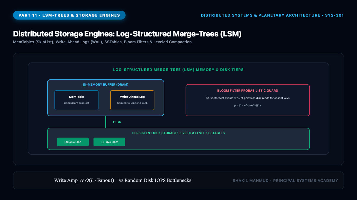
Traditional relational databases relied on in-place update structures, notably the classical B-Tree (Bayer & McCreight, 1972). While B-Trees offer optimal read latencies ($mathcal{O}(log N)$ page accesses), concurrent random disk writes incur catastrophic write amplification and severe random I/O bottlenecks. In 1996, Patrick O’Neil, Edward O’Neil, and Gerhard Weikum introduced the Log-Structured Merge-Tree (LSM-Tree). By converting random writes into high-throughput sequential appends and deferring sorting to background asynchronous compaction, LSM-trees became the standard storage engine powering distributed massive-scale databases, including Google Bigtable, Apache Cassandra, RocksDB, ScyllaDB, and TiKV.
1. The Write-Path Architecture: From Memory to Immutable SSTables
An LSM-tree architecture bifurcates the lifecycle of mutated data into high-speed volatile memory structures and immutable on-disk files:
1. The Write-Ahead Log (WAL) & MemTable
When a client issues a write (`Put(k, v)` or `Delete(k)`):
- The mutation is immediately appended sequentially to an on-disk Write-Ahead Log (WAL). Because this is a strictly sequential append without disk seeks, write throughput reaches physical NVMe/SSD interface bandwidth. The WAL guarantees crash durability.
- Concurrently, the key-value pair is inserted into an in-memory sorted structure known as the MemTable (typically implemented as a lock-free SkipList or Red-Black Tree). Deletions are inserted as special marker entries called Tombstones.
- The write returns success to the client with sub-millisecond latency.
2. MemTable Flushing to L0 SSTables
When the active MemTable exceeds a configured memory threshold (e.g. 64 MB), it transitions to an Immutable MemTable, and a fresh active MemTable is allocated. A background I/O thread flushes the immutable MemTable sequentially to disk as a Sorted String Table (SSTable) at Level 0 ($L_0$), and the corresponding WAL segment is reclaimed.
2. Anatomy of an SSTable
An SSTable is a strictly immutable, sequentially sorted file organized into four internal components:
- Data Blocks: Contiguous fixed-size blocks (typically 4 KB – 64 KB) containing ordered key-value pairs, compressed with LZ4 or Zstandard. Delta encoding is used on adjacent keys to maximize compression ratios.
- Block Index: A sparse index stored at the end of the file mapping the first key of each data block to its physical byte offset within the file. Reading a key requires loading only this sparse index into RAM, finding the candidate block via binary search, and seeking directly to that single data block.
- Bloom Filter: A probabilistic bit array that eliminates unnecessary disk seeks for non-existent keys.
- Footer: Fixed-size trailing metadata storing byte offsets and checksums for the block index and Bloom filter.
3. Mathematical Optimization: Bloom Filters
Because keys are scattered across multiple immutable SSTables, reading a non-existent key could force disk lookups across every SSTable in the database. LSM-trees eliminate this via Bloom Filters.
Given an SSTable with $n$ keys and a bit array of size $m$ using $k$ independent uniform hash functions $h_1, h_2, dots, h_k$:
- Insertion: For each key $x$, set bits at indices $h_1(x), dots, h_k(x)$ to $1$.
- Query: Key $y$ is tested at all $k$ bit indices. If any bit is $0$, the key is guaranteed not to exist in the SSTable (zero false negatives).
The optimal number of hash functions $k$ that minimizes the false positive probability $p$ is:
$$k = rac{m}{n} ln 2 pprox 0.693 rac{m}{n}$$
Under this optimal $k$, the false positive rate decays exponentially with the bits-per-key ratio $m/n$:
$$p pprox left( rac{1}{2}
ight)^k = (0.6185)^{m/n}$$
Allocating just 10 bits per key ($m/n = 10$) with $k = 7$ hash functions yields a false positive rate of approximately $0.99%$—filtering out over $99%$ of redundant disk reads in memory.
4. Background Compaction: Leveled vs. Size-Tiered
As SSTables accumulate, read performance degrades and stale/deleted data consumes disk space. LSM-trees resolve this via Compaction—merging multiple SSTables into a single sorted SSTable via a continuous $k$-way merge sort, discarding overwritten versions and tombstones.
Size-Tiered Compaction Strategy (STCS)
STCS groups SSTables of similar sizes into tiers. When a tier accumulates $N$ SSTables (e.g. 4), they are merged into a single larger SSTable in the next tier.
- Advantage: Fast writes; minimal background I/O overhead.
- Disadvantage: High space amplification (can require up to $50%$ free disk space to complete large merges) and inconsistent read latencies. Ideal for write-heavy append workloads (Cassandra).
Leveled Compaction Strategy (LCS)
LCS organizes files into discrete levels ($L_0, L_1, L_2, dots$), where the total capacity of level $L_{i+1}$ is exponentially larger than $L_i$ (typically $10 imes$):
$$ ext{Capacity}(L_i) = 10^i imes ext{BaseSize}$$
Crucially, in levels $L_1$ and above, key ranges between SSTables within the same level never overlap. When level $L_i$ exceeds its quota, an SSTable is chosen and merged with all overlapping SSTables in $L_{i+1}$.
- Advantage: Exceptional read latency (at most one SSTable lookup per level), tight space amplification ($pprox 10%$), and deterministic disk footprint.
- Trade-off: Higher write amplification, heavily optimized in RocksDB and CockroachDB.