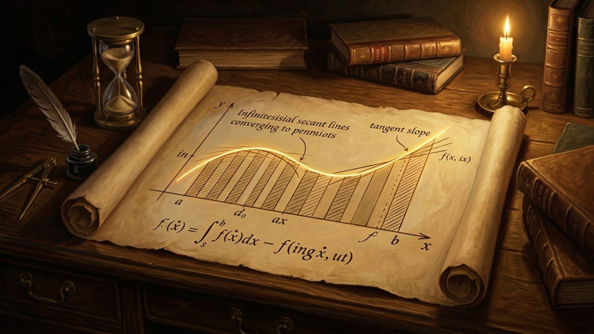
Before the mid-seventeenth century, mathematics was fundamentally static. Ancient Euclidean geometry and Apollonian conic sections could describe circles, triangles, and ellipses in eternal resting equilibrium, but the real universe is a symphony of relentless change: a cannonball decelerating against atmospheric drag, planets accelerating along gravitational gradients, and heat diffusing through an iron bar. For two millennia, natural philosophy had suffered from a profound schism: one group of thinkers studied the geometric problem of finding the tangent slope to a curved line, while another studied the problem of calculating the curved area beneath a shape. It was the crowning intellectual achievement of Isaac Newton and Gottfried Wilhelm Leibniz to demonstrate that these two separate enigmas were, in fact, mirror images of the exact same process: The Fundamental Theorem of Calculus.
1. The Dichotomy: Tangents versus Quadratures
In classical geometry, calculating the tangent to a curve was a problem of differentiation: what is the instantaneous rate of change of a function $f(x)$ at an exact moment? If a falling body moves according to position $s(t)$, what is its velocity at precisely $t = 3.0$ seconds without dividing zero by zero?
Conversely, finding the area under a curve was a problem of integration (then called quadrature). Archimedes had approached this through the grueling “method of exhaustion,” inscribing ever-narrower polygons inside parabolas. Pierre de Fermat and René Descartes had advanced the techniques, but each new curve required a bespoke, heroic geometric tour de force.
Newton and Leibniz recognized that instantaneous rate and accumulated sum are exact inverse operations. As formalized mathematically:
$$frac{d}{dx} left( int_a^x f(t),dt right) = f(x)$$
$$int_a^b f(x),dx = F(b) – F(a) quad text{where } F'(x) = f(x)$$
The second part of the theorem is what liberated science: to find the total accumulated area under any continuous curve, one does not need to sum an infinity of vanishing trapezoids; one only needs to find the antiderivative function $F(x)$ and evaluate it at the endpoints.
2. Newton’s Fluxions versus Leibniz’s Differentials
Between 1665 and 1666, isolated at Woolsthorpe Manor during the Great Plague of London, Isaac Newton developed his “Method of Fluxions.” He viewed variables as “fluents” generated by continuous motion, and their velocities as “fluxions” denoted by dotted letters ($dot{x}, dot{y}$).
A decade later in Paris, working independently, Gottfried Wilhelm Leibniz approached the problem from the perspective of symbolic logic and discrete differences. Leibniz invented the enduring notation that still graces every physics chalkboard today: the elongated Latin ‘S’ for summation ($int$) and the differential operator ($d$ for differentia):
$$frac{dy}{dx} = lim_{Delta x to 0} frac{f(x + Delta x) – f(x)}{Delta x}$$
While Newton viewed calculus as a physical tool to derive celestial gravitation, Leibniz realized that notation dictates thought. His quotient notation $frac{dy}{dx}$ and product rule $d(uv) = u,dv + v,du$ made advanced multi-step derivations almost mechanical, sparking the explosive flowering of mathematical analysis across continental Europe led by the Bernoulli family and Leonhard Euler.
3. The Architecture of Modern Deep Learning: The Chain Rule and Gradient Descent
Today, calculus is not merely the operating system of classical physics, aerodynamics, and quantum mechanics; it is the algorithmic engine powering modern Artificial Intelligence.
Every Large Language Model, neural network, and autonomous vehicle learns by minimizing an objective loss function $mathcal{L}(theta)$. To train a model containing hundreds of billions of synaptic parameters, the algorithm propagates error signals backward through deep hierarchical computational layers using the multivariable Chain Rule of Calculus:
$$frac{partial mathcal{L}}{partial w_{ij}} = frac{partial mathcal{L}}{partial a_j} cdot frac{partial a_j}{partial z_j} cdot frac{partial z_j}{partial w_{ij}}$$
Parameters are updated iteratively along the negative gradient of the loss surface via gradient descent:
$$theta_{t+1} = theta_t – eta nabla_theta mathcal{L}(theta)$$
Without the Fundamental Theorem of Calculus, the continuous optimization of neural weights, the simulation of rocket trajectories, and the modeling of planetary climate would be utterly impossible.