How do high-energy particle accelerators like the Large Hadron Collider at CERN translate microscopic Lagrangian symmetries into measurable physical cross-sections? The answer lies in the Scattering Matrix ($S$-Matrix) and Richard Feynman’s iconic pictorial calculus: Feynman Diagrams. By mapping intricate multi-dimensional perturbation integrals into intuitive topological networks of propagating particles and interacting vertices, Feynman revolutionized quantum calculations, turning unsolvable differential equations into elegant algebraic rules.
1. The S-Matrix and Dyson’s Expansion
In a typical particle collider experiment, particles are prepared in asymptotically free states at $t to -infty$, collide in a compact interaction region, and scatter into free outgoing states at $t to +infty$. The unitary $S$-matrix connects initial states $|irangle$ to final states $|frangle$:
[
S_{fi} equiv langle f | S | i rangle = langle f | U(+infty, -infty) | i rangle
]
In the interaction picture, the time-evolution operator is given by the time-ordered exponential known as Dyson’s Formula:
[
S = T left{ expleft( -i int_{-infty}^infty dt , H_{text{int}}(t) right) right} = sum_{n=0}^infty frac{(-i)^n}{n!} int d^4x_1 dots d^4x_n , T{ mathcal{H}_{text{int}}(x_1) dots mathcal{H}_{text{int}}(x_n) }
]
Separating the trivial non-interacting forward-scattering identity $S = I + i T$ defines the Transition Matrix $T$. Factoring out 4-momentum conservation yields the invariant scattering amplitude $mathcal{M}$:
[
langle f | i T | i rangle = (2pi)^4 delta^{(4)}left( sum p_f – sum p_i right) i mathcal{M}_{fi}
]
2. Wick’s Theorem: Contractions into Propagators
Evaluating Dyson’s time-ordered products of quantum field operators directly is algebraically intractable. Gian-Carlo Wick proved that any time-ordered product of free fields is identically equal to its normal-ordered product plus all possible pairwise Feynman Contractions:
[
T{ phi(x_1) dots phi(x_n) } = : phi(x_1) dots phi(x_n) : + sum_{text{contractions}} : phi(x_1) dots overbrace{phi(x_i) dots phi(x_j)}^{bullet} dots phi(x_n) :
]
where the contraction of two field operators is precisely the c-number Feynman Propagator:
[
overbrace{phi(x)phi(y)}^{bullet} equiv langle 0 | T{phi(x)phi(y)} | 0 rangle = Delta_F(x – y)
]
When sandwiched between the vacuum $langle 0 | dots | 0 rangle$, all normal-ordered terms vanish identically, leaving purely the fully contracted Feynman propagators.
3. Tree-Level Møller Scattering in QED
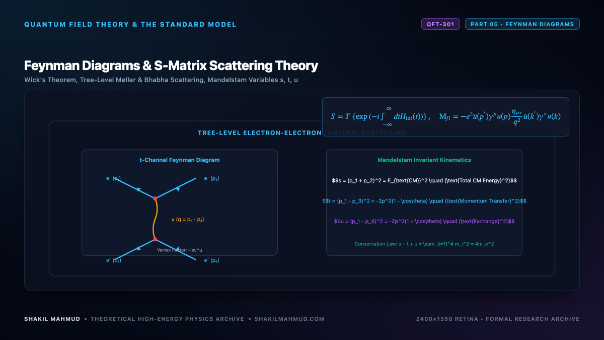
Applying Wick’s theorem to electron-electron (Møller) scattering ($e^- e^- to e^- e^-$) at second order ($mathcal{O}(e^2)$), two distinct Feynman diagrams contribute:
- The $t$-Channel Direct Exchange: A photon of momentum $q = p_1 – p_3$ is exchanged between the two electron currents.
- The $u$-Channel Exchange: Fermi-Dirac statistics require an identical diagram with the final electrons swapped ($p_3 leftrightarrow p_4$), entering with a relative minus sign.
Using the Feynman rules for QED, the tree-level invariant amplitude is expressed directly as:
[
i mathcal{M} = (-i e)^2 left[ frac{bar{u}(p_3) gamma^mu u(p_1) , eta_{munu} , bar{u}(p_4) gamma^nu u(p_2)}{(p_1 – p_3)^2} – frac{bar{u}(p_4) gamma^mu u(p_1) , eta_{munu} , bar{u}(p_3) gamma^nu u(p_2)}{(p_1 – p_4)^2} right]
]
4. Mandelstam Invariants and Relativistic Cross-Sections
To analyze scattering kinematics covariantly, Stanley Mandelstam defined three relativistic Lorentz-invariant variables for a $2 to 2$ process ($p_1 + p_2 to p_3 + p_4$):
[
begin{aligned}
s &equiv (p_1 + p_2)^2 = E_{text{CM}}^2 quad (text{Center-of-Mass Energy Squared}) \
t &equiv (p_1 – p_3)^2 = -2 p_{text{CM}}^2 (1 – costheta) quad (text{Momentum Transfer Squared}) \
u &equiv (p_1 – p_4)^2 = -2 p_{text{CM}}^2 (1 + costheta) quad (text{Cross-Exchange Squared})
end{aligned}
]
Energy-momentum conservation strictly enforces the universal kinematic identity:
[
s + t + u = m_1^2 + m_2^2 + m_3^2 + m_4^2
]
Integrating the spin-averaged squared amplitude $|overline{mathcal{M}}|^2$ over Lorentz-invariant phase space yields the differential cross-section:
[
frac{dsigma}{dOmega} = frac{1}{64pi^2 s} |overline{mathcal{M}}|^2
]
This bridges abstract quantum field operators to the exact detector counts recorded in experimental particle physics.