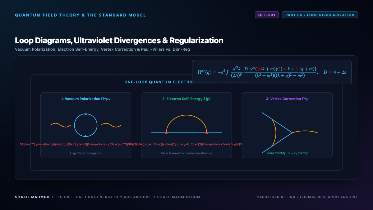
When physicists in the late 1940s computed higher-order corrections to tree-level Feynman diagrams, they were horrified to discover that closed virtual particle loops produced nonsensical mathematical infinities. Because virtual particles circulating in a closed loop can possess arbitrarily large 4-momentum $k^mu to infty$, the corresponding momentum-space loop integrals diverge in the ultraviolet (UV) regime. Taming these infinities without violating Poincaré symmetry or local gauge invariance required the development of Regularization Theory, culminating in Gerard ‘t Hooft and Martinus Veltman’s Nobel-winning method of Dimensional Regularization.
1. The Origin of Ultraviolet Divergences in Loops
In any Feynman diagram containing $L$ closed loops, energy-momentum conservation fixes all internal momenta except for $L$ undetermined loop 4-momenta $k_l$. Consider the 1-loop electron self-energy diagram in QED, where an electron emits and reabsorbs a virtual photon. The integral takes the form:
[
-i Sigma(p) = (-ie)^2 int frac{d^4k}{(2pi)^4} gamma^mu frac{i(sl k + m)}{k^2 – m^2 + ivarepsilon} gamma_mu frac{-i}{(p – k)^2 + ivarepsilon}
]
For large loop momentum $k to infty$, the numerator scales as $sim k$ while the denominator scales as $sim k^4$. The integral behaves asymptotically as:
[
int^Lambda frac{k^3 , dk cdot k}{k^4} sim int^Lambda dk sim Lambda quad (text{Linearly Divergent})
]
Similarly, the photon vacuum polarization loop $Pi^{munu}(q)$ diverges quadratically $sim Lambda^2$, threatening the masslessness of the photon and violating gauge invariance if cut off naively with a hard momentum threshold $|k| le Lambda$.
2. Feynman Parameterization
To integrate denominators containing products of disparate momentum factors, we utilize Feynman’s Parameterization Identity:
[
frac{1}{A B} = int_0^1 dx frac{1}{left[ x A + (1 – x) B right]^2}
]
Shifting the integration variable to $l = k – x p$ combines denominators into a symmetric spherically invariant form $left( l^2 – Delta right)^{-2}$, where $Delta = x m^2 – x(1-x)p^2$.
3. Dimensional Regularization ($D = 4 – 2varepsilon$)
The breakthrough technique introduced by ‘t Hooft and Veltman in 1972 is to evaluate loop integrals in an arbitrary complex spacetime dimension $D$. Defining $varepsilon equiv frac{4 – D}{2}$, the spacetime volume element transforms as:
[
int frac{d^4k}{(2pi)^4} longrightarrow mu^{2varepsilon} int frac{d^D k}{(2pi)^D}
]
where $mu$ is an arbitrary ‘t Hooft energy scale introduced to preserve the dimensionless nature of the coupling constant $e$. Performing the $D$-dimensional Euclidean angular integration using Euler Gamma functions $Gamma(z)$ yields the master integral:
[
int frac{d^D l}{(2pi)^D} frac{1}{(l^2 – Delta)^n} = frac{(-1)^n i}{(4pi)^{D/2}} frac{Gammaleft(n – frac{D}{2}right)}{Gamma(n)} Delta^{frac{D}{2} – n}
]
Near $D = 4$ ($n=2$), expanding the Gamma function via Laurent series $Gamma(varepsilon) = frac{1}{varepsilon} – gamma_E + mathcal{O}(varepsilon)$ isolates the ultraviolet infinity cleanly into an explicit simple pole:
[
mu^{2varepsilon} int frac{d^D l}{(2pi)^D} frac{1}{(l^2 – Delta)^2} = frac{i}{16pi^2} left[ frac{1}{varepsilon} – gamma_E + lnleft( frac{4pi mu^2}{Delta} right) + mathcal{O}(varepsilon) right]
]
4. Preservation of Ward Identities
Because dimensional regularization involves no hard momentum boundary cutoff $Lambda$, translational invariance in momentum space $int d^D k f(k) = int d^D k f(k + p)$ is rigorously preserved. Consequently, the vacuum polarization tensor satisfies the transversality condition automatically:
[
q_mu Pi^{munu}(q) = 0 implies Pi^{munu}(q) = (q^2 eta^{munu} – q^mu q^nu) Pi(q^2)
]
The photon remains strictly massless at all loop orders, preserving the Ward-Takahashi identity and the local $U(1)$ gauge symmetry of Quantum Electrodynamics.