A dynamical system is rarely rigid; its governing equations depend on physical parameters—temperatures, flow velocities, chemical affinities, voltages. As a parameter smoothly varies, the system usually responds with smooth quantitative deformation. However, at certain critical thresholds, the qualitative topological structure of the phase portrait abruptly fractures: fixed points collide, exchange stability, or split into existence. This geometric metamorphosis is Bifurcation Theory.
1. Structural Stability & Codimension-1 Bifurcations
A parameterized dynamical system $dot{mathbf{x}} = mathbf{f}(mathbf{x}, r)$ is structurally stable if small perturbations in the parameter $r$ leave the qualitative topology of the phase space portrait unchanged (i.e., there exists a trajectory-preserving homeomorphism between portraits before and after the change). Points in parameter space where structural stability breaks down are Bifurcation Points ($r = r_c$).
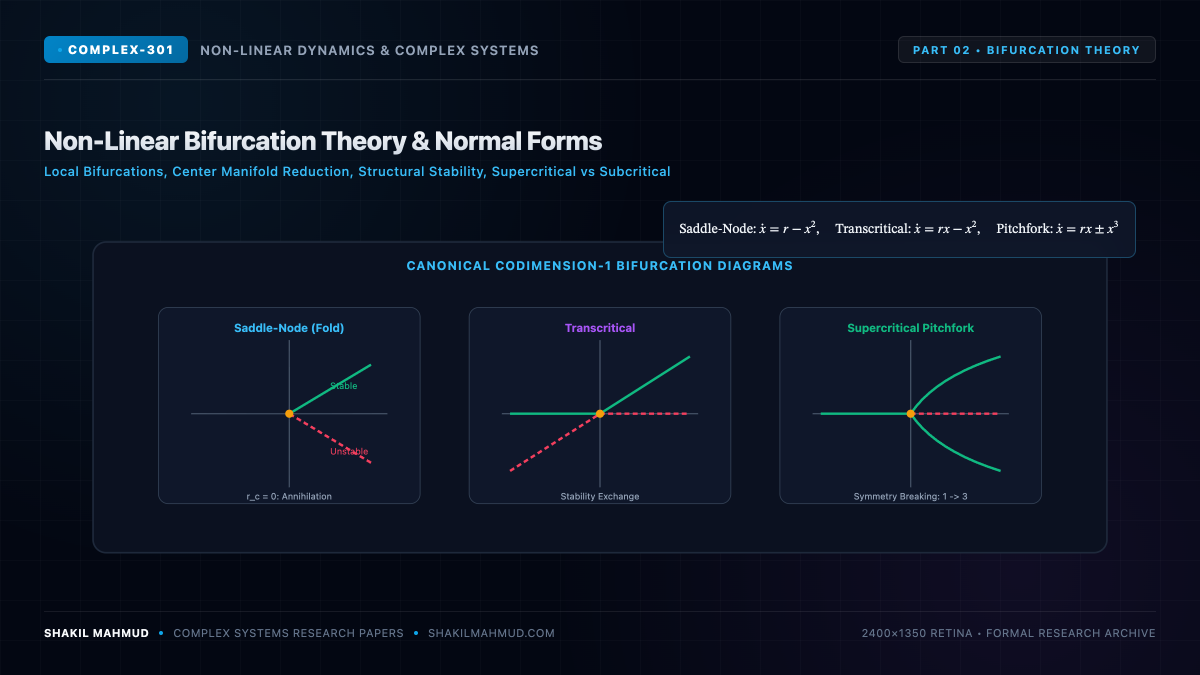
The codimension of a bifurcation is the minimum number of independent control parameters that must be tuned to encounter it. In a one-parameter family ($r in mathbb{R}$), there are three canonical local codimension-1 bifurcations of fixed points in one dimension:
2. The Three Fundamental Local Bifurcations
A. Saddle-Node (Fold / Limit Point) Bifurcation
The saddle-node bifurcation represents the basic mechanism by which equilibria are born or annihilated. Its canonical Normal Form is:
[
dot{x} = r – x^2
]
Analyzing the roots $r – x^2 = 0$:
- $r < 0$: No real fixed points exist; the vector field is everywhere negative ($dot{x} < 0$), and trajectories drift to $-infty$.
- $r = 0$: A single half-stable degenerate fixed point appears at $x^* = 0$ with eigenvalue $lambda = f'(0) = 0$.
- $r > 0$: The point splits into two distinct fixed points: a stable node at $x^*_{text{stable}} = +sqrt{r}$ ($lambda = -2sqrt{r} 0$).
B. Transcritical Bifurcation
Occurring frequently in ecology, epidemiology, and laser physics, fixed points in a transcritical bifurcation never disappear; instead, they collide and exchange stability. The normal form is:
[
dot{x} = r x – x^2 = x(r – x)
]
The fixed points are $x_1^* = 0$ and $x_2^* = r$:
- For $r < 0$, $x_1^* = 0$ is stable ($lambda = r 0$).
- At $r = 0$, the two points collide into a single non-hyperbolic equilibrium.
- For $r > 0$, $x_1^* = 0$ becomes unstable ($lambda = r > 0$) while $x_2^* = r$ becomes stable ($lambda = -r < 0$). Stability has been transferred between the branches.
C. Pitchfork Bifurcations: Symmetry Breaking
When a physical system possesses reflection symmetry (invariant under spatial inversion $x to -x$), the governing vector field must be an odd function ($f(-x) = -f(x)$). Pitchfork bifurcations govern the spontaneous breakdown of spatial symmetry.
- Supercritical Pitchfork: Normal form:
[
dot{x} = r x – x^3
]
For $r le 0$, the origin $x^* = 0$ is the unique stable equilibrium. As $r$ increases above $0$, the origin destabilizes ($lambda = r > 0$), and two symmetric, stable off-axis fixed points emerge: $x^* = pmsqrt{r}$. This models spontaneous magnetization in the Curie-Weiss ferromagnetic transition. - Subcritical Pitchfork: Normal form:
[
dot{x} = r x + x^3 – x^5
]
Here, the emerging branches $x^* = pmsqrt{-r}$ for $r < 0$ are unstable. When $r$ crosses $0$, the origin loses stability violently, forcing trajectories to jump discontinuously to distant large-amplitude attractors—exhibiting hysteresis and dangerous tipping points characteristic of structural buckling and catastrophic ecosystem collapse.
3. Center Manifold Reduction
How do we analyze bifurcations in high-dimensional systems ($mathbb{R}^n$ with $n gg 1$)?
According to the Center Manifold Theorem, near a bifurcation point, the phase space decomposes into three invariant submanifolds corresponding to the stable ($text{Re}(lambda) 0$), and center ($text{Re}(lambda) = 0$) eigenspaces. Because the stable directions decay exponentially fast, the essential asymptotic dynamics of the entire $n$-dimensional system contract onto the low-dimensional Center Manifold $W^c$, allowing complex non-linear networks to be rigorously reduced to simple one- or two-dimensional normal forms.