At the foundation of modern non-linear dynamics lies a geometric conceptual revolution inaugurated by Henri Poincaré: instead of seeking unattainable closed-form analytical solutions to non-linear differential equations, we investigate the global geometric and topological properties of trajectories moving through continuous Phase Space under the action of deterministic vector fields.
1. Dynamical Systems as Vector Fields & Flows
An autonomous continuous dynamical system in an $n$-dimensional state space $mathcal{M} subseteq mathbb{R}^n$ is defined by a system of first-order ordinary differential equations (ODEs):
[
dot{mathbf{x}} = frac{dmathbf{x}}{dt} = mathbf{f}(mathbf{x}), quad mathbf{x} in mathbb{R}^n, quad mathbf{f}: mathbb{R}^n to mathbb{R}^n
]
The vector field $mathbf{f}(mathbf{x})$ assigns a velocity vector to every point in phase space. The integrated time evolution generates a one-parameter group of diffeomorphisms known as the Phase Flow $phi_t: mathcal{M} to mathcal{M}$, satisfying:
- $phi_0(mathbf{x}) = mathbf{x}$ (Identity mapping at $t = 0$).
- $phi_{t + s}(mathbf{x}) = phi_t(phi_s(mathbf{x}))$ for all $t, s in mathbb{R}$ (Group composition law).
By the Picard-Lindelöf Existence and Uniqueness Theorem, if the vector field $mathbf{f}$ is continuously differentiable ($mathcal{C}^1$), then through every initial point $mathbf{x}_0 in mathcal{M}$ passes one and only one trajectory $mathbf{x}(t) = phi_t(mathbf{x}_0)$. A direct topological consequence of this theorem is that trajectories in autonomous phase space can never intersect, cross, or split; two distinct paths can never occupy the same state at the same time.
2. Equilibrium States & The Jacobian Matrix
A point $mathbf{x}^* in mathcal{M}$ where the velocity field vanishes is termed a Fixed Point (Equilibrium / Singular Point):
[
mathbf{f}(mathbf{x}^*) = mathbf{0}
]
To analyze the local stability of an equilibrium point, we linearize the system about $mathbf{x}^*$ by considering an infinitesimal perturbation $boldsymbol{xi}(t) = mathbf{x}(t) – mathbf{x}^*$. Performing a Taylor expansion:
[
dot{boldsymbol{xi}} = mathbf{f}(mathbf{x}^* + boldsymbol{xi}) = mathbf{f}(mathbf{x}^*) + J(mathbf{x}^*) boldsymbol{xi} + mathcal{O}(|boldsymbol{xi}|^2) approx J(mathbf{x}^*) boldsymbol{xi}
]
Where $J(mathbf{x}^*) = nabla mathbf{f}(mathbf{x}^*)$ is the $n times n$ Jacobian Matrix of first partial derivatives:
[
J_{ij} = left. frac{partial f_i}{partial x_j} right|_{mathbf{x} = mathbf{x}^*}
]
The solution to the linearized variational equation is given by matrix exponentiation:
[
boldsymbol{xi}(t) = exp(J t) boldsymbol{xi}(0) = sum_{k=1}^n c_k e^{lambda_k t} mathbf{v}_k
]
Where $lambda_k$ are the complex eigenvalues and $mathbf{v}_k$ are the corresponding eigenvectors satisfying the characteristic polynomial $det(J – lambda I) = 0$.
3. Classification of Planar Singularities ($mathbb{R}^2$)
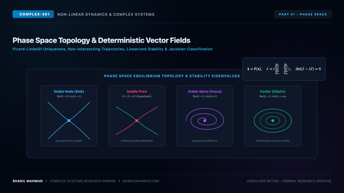
In a two-dimensional phase plane ($n = 2$), the Jacobian has trace $tau = text{Tr}(J) = lambda_1 + lambda_2$ and determinant $Delta = det(J) = lambda_1 lambda_2$. The characteristic equation becomes $lambda^2 – tau lambda + Delta = 0$, with eigenvalues:
[
lambda_{1, 2} = frac{tau pm sqrt{tau^2 – 4Delta}}{2}
]
The topological nature of the equilibrium point is governed by the discriminant $delta = tau^2 – 4Delta$:
| Topological Class | Determinant $Delta$ | Trace $tau$ | Discriminant $delta$ | Eigenvalues $lambda_{1,2}$ | Stability Character |
|---|---|---|---|---|---|
| Saddle Point | $Delta < 0$ | Any | $delta > 0$ | $lambda_1 < 0 < lambda_2$ (Real, opposite sign) | Unstable (Hyperbolic) |
| Stable Node (Sink) | $Delta > 0$ | $tau < 0$ | $delta ge 0$ | $lambda_2 le lambda_1 < 0$ (Real, negative) | Asymptotically Stable |
| Unstable Node (Source) | $Delta > 0$ | $tau > 0$ | $delta ge 0$ | $lambda_1 ge lambda_2 > 0$ (Real, positive) | Unstable |
| Stable Spiral (Focus) | $Delta > 0$ | $tau < 0$ | $delta < 0$ | $alpha pm iomega, ; alpha < 0$ | Asymptotically Stable (Damped) |
| Unstable Spiral (Focus) | $Delta > 0$ | $tau > 0$ | $delta < 0$ | $alpha pm iomega, ; alpha > 0$ | Unstable (Amplifying) |
| Center (Elliptic) | $Delta > 0$ | $tau = 0$ | $delta < 0$ | $pm iomega$ (Pure imaginary) | Neutrally Stable (Conservative) |
4. The Hartman-Grobman Theorem
When does linear stability accurately reflect the true non-linear reality? The answer is formalized by the Hartman-Grobman Theorem:
If an equilibrium point $mathbf{x}^*$ is hyperbolic—meaning none of the eigenvalues of the Jacobian matrix have zero real parts ($text{Re}(lambda_k) neq 0$ for all $k$)—then there exists a local neighborhood $U$ of $mathbf{x}^*$ and a homeomorphism $h: U to V$ that maps the non-linear trajectories of $dot{mathbf{x}} = mathbf{f}(mathbf{x})$ bijectively and continuously onto the linear trajectories of $dot{boldsymbol{xi}} = J boldsymbol{xi}$.
Thus, non-linear effects cannot alter the qualitative topological portrait of a hyperbolic fixed point; linearization is rigorous and exact. However, when $text{Re}(lambda) = 0$ (such as in centers or bifurcation points), higher-order non-linear terms dictate the global qualitative dynamics.