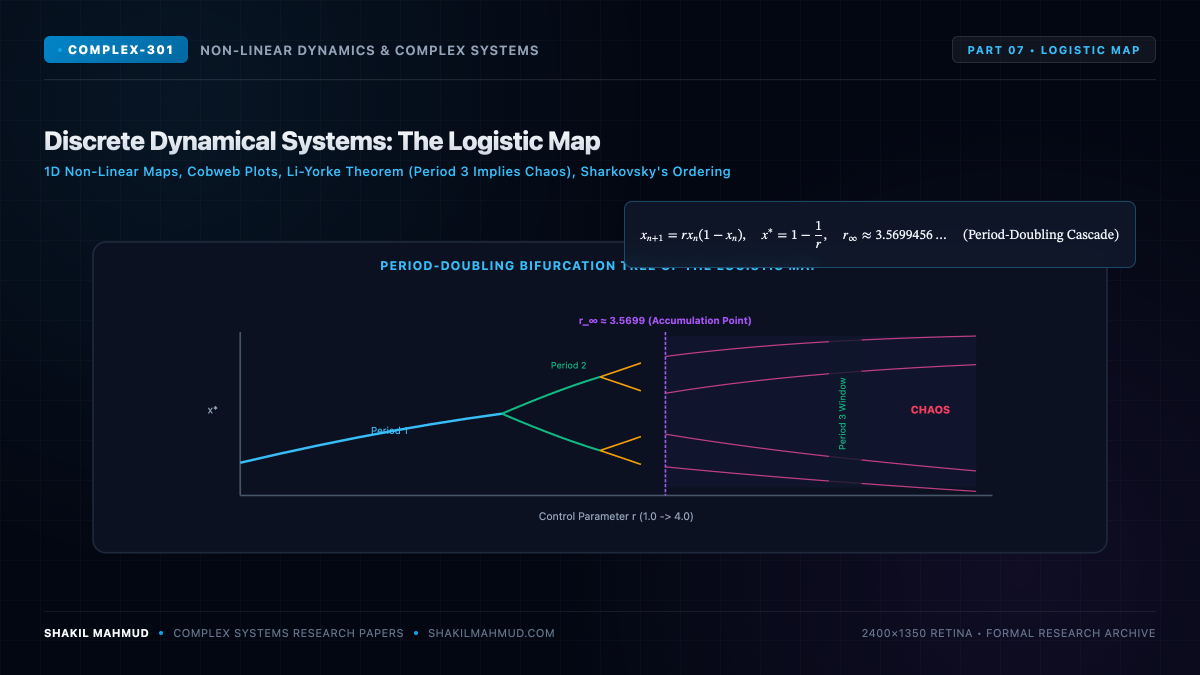
While continuous differential equations require at least three dimensions to exhibit chaos, discrete difference equations can generate boundless chaotic complexity in a single spatial dimension ($n = 1$). The iconic crucible of 1D non-linear dynamics is the Logistic Map, popularized by theoretical ecologist Robert May in 1976 as a masterclass in how simple non-linear algebraic models produce mathematical universes.
1. The Geometry of Iterated 1D Maps
The logistic difference equation models population dynamics under carrying-capacity saturation:
[
x_{n+1} = f(x_n) = r x_n (1 – x_n)
]
Where $x_n in [0, 1]$ represents the normalized population density in generation $n$, and $r in [0, 4]$ is the non-linear growth parameter. The geometric evolution of iterations can be visualized via Cobweb Diagrams: plotting the parabolic function $y = f(x)$ alongside the diagonal identity reflection line $y = x$.
2. Fixed Points & Stability Multipliers
The fixed points satisfy $x^* = f(x^*) = r x^*(1 – x^*)$. Solving algebraically yields two solutions:
- $x_0^* = 0$ (Extinction equilibrium).
- $x_1^* = 1 – frac{1}{r}$ (Carrying-capacity survival equilibrium, existing for $r > 1$).
The stability of a fixed point in a 1D map is determined not by eigenvalues, but by the magnitude of the Multiplier $mu = f'(x^*)$:
[
f'(x) = r(1 – 2x) implies f'(x_1^*) = rleft(1 – 2left(1 – frac{1}{r}right)right) = 2 – r
]
By linear stability theory for difference equations:
- If $|f'(x^*)| < 1$, the fixed point is linearly attracting (stable).
- If $|f'(x^*)| > 1$, the fixed point is linearly repelling (unstable).
- If $f'(x^*) = -1$, a flip (period-doubling) bifurcation occurs.
Setting $|2 – r| < 1$ demonstrates that $x_1^*$ is stable in the interval $1 < r < 3$.
3. The Period-Doubling Pitchfork Cascade
What happens when $r$ exceeds $3$? At $r_1 = 3$, the multiplier hits $f'(x_1^*) = -1$. The fixed point destabilizes and sheds a stable 2-cycle ($x_{a} leftrightarrow x_{b}$), which are fixed points of the second iterate $f^{(2)}(x) = f(f(x))$.
As $r$ continues to increase, the 2-cycle in turn destabilizes at $r_2 = 1 + sqrt{6} approx 3.449$, splitting into a stable 4-cycle. This triggers an infinite, geometric cascade of period-doublings:
[
2^0 xrightarrow{r_1 = 3.0} 2^1 xrightarrow{r_2 approx 3.449} 2^2 xrightarrow{r_3 approx 3.544} 2^3 xrightarrow{r_4 approx 3.564} dots longrightarrow 2^infty
]
The sequence of bifurcation parameter values $r_n$ converges geometrically to a finite limit known as the Accumulation Point:
[
r_infty approx 3.569945672dots
]
Beyond $r_infty$, the system enters the fully chaotic regime, where orbits wander ergodically through dense fractal bands without ever settling onto a periodic pattern.
4. Li-Yorke Theorem & Sharkovsky’s Ordering
Within the chaotic sea ($r > r_infty$), stable periodic windows unexpectedly re-emerge. Most famously, at $r approx 3.8284$, a prominent Period-3 Window opens.
In 1975, Tien-Yien Li and James A. Yorke published their landmark theorem: “Period Three Implies Chaos.” They proved rigorously that for any continuous 1D interval map $f: I to I$, if there exists an orbit of period 3, then:
- The map possesses periodic orbits of every integer period $k = 1, 2, 3, 4, 5, dots$.
- There exists an uncountably infinite set of initial states (the scrambled set) whose trajectories exhibit aperiodic deterministic chaos.
This result is unified by Sharkovsky’s Theorem (1964), which ordered all natural numbers in a remarkable hierarchy:
[
3 rhd 5 rhd 7 rhd 9 rhd dots rhd 2 cdot 3 rhd 2 cdot 5 rhd dots rhd 2^2 cdot 3 rhd dots rhd 2^3 rhd 2^2 rhd 2 rhd 1
]
If a continuous map has an orbit of period $p$, it is mathematically guaranteed to possess orbits of all periods $q$ appearing to the right of $p$ in Sharkovsky’s ordering ($p rhd q$). Because $3$ sits at the absolute throne of the hierarchy, the existence of period 3 implies everything!