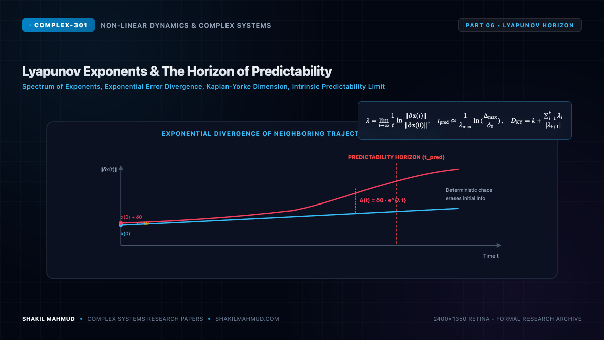
How do we mathematically quantify “chaos”? Qualitative assertions of unpredictability are made rigorous by the spectrum of Lyapunov Exponents—the asymptotic rates of exponential divergence or convergence of infinitesimally close trajectories in phase space. The existence of at least one positive Lyapunov exponent is the unambiguous diagnostic signature of deterministic chaos, establishing a hard, unbreachable physical Horizon of Predictability.
1. The Variational Equations & Tangent Space Dynamics
Consider an autonomous dynamical system $dot{mathbf{x}} = mathbf{f}(mathbf{x})$ on $mathbb{R}^n$. Let $mathbf{x}(t)$ be a reference trajectory and $mathbf{y}(t) = mathbf{x}(t) + boldsymbol{delta}(t)$ be a nearby trajectory initialized with an infinitesimal separation vector $boldsymbol{delta}(0) in T_{mathbf{x}(0)} mathcal{M}$ in the tangent space.
The time evolution of the separation vector $boldsymbol{delta}(t)$ is governed by the linearized Variational Equation:
[
dot{boldsymbol{delta}}(t) = J(mathbf{x}(t)) boldsymbol{delta}(t) = left. nabla mathbf{f} right|_{mathbf{x}(t)} boldsymbol{delta}(t)
]
The fundamental solution operator $M(t, mathbf{x}_0)$ maps initial tangent vectors to their state at time $t$:
[
boldsymbol{delta}(t) = M(t, mathbf{x}_0) boldsymbol{delta}(0)
]
By the Oseledec Multiplicative Ergodic Theorem (1968), for almost every initial condition with respect to an ergodic invariant measure, the asymptotic limit of the symmetric positive-definite matrix:
[
Lambda(mathbf{x}_0) = lim_{t to infty} left[ M(t, mathbf{x}_0)^T M(t, mathbf{x}_0) right]^{1 / 2t}
]
exists. The natural logarithms of the eigenvalues of $Lambda(mathbf{x}_0)$ define the ordered Lyapunov Spectrum:
[
lambda_1 ge lambda_2 ge dots ge lambda_n
]
2. Maximal Lyapunov Exponent & Algorithmic Calculation
The Maximal Lyapunov Exponent (MLE) $lambda_{max} = lambda_1$ governs the long-term separation of generic initial perturbations:
[
lambda_{max} = lim_{t to infty} frac{1}{t} ln left( frac{|boldsymbol{delta}(t)|}{|boldsymbol{delta}(0)|} right)
]
- $lambda_{max} < 0$: Trajectories converge asymptotically to a single stable fixed point.
- $lambda_{max} = 0$: Trajectories lie on a stable periodic limit cycle or quasi-periodic torus. (In any continuous autonomous flow without fixed points, the exponent along the direction of the flow is always identically zero: $lambda_{text{flow}} = 0$).
- $lambda_{max} > 0$: Neighboring trajectories separate exponentially fast—the definitive mathematical definition of deterministic chaos.
In numerical computations, tracking tangent vectors directly causes numerical overflow due to exponential growth. In 1980, Giancarlo Benettin and colleagues formulated the standard numerical algorithm: integrating the variational equations alongside periodic Gram-Schmidt re-orthonormalization at discrete time intervals $tau$, accumulating the stretching logs $lambda_k approx frac{1}{Ktau} sum_{m=1}^K ln |mathbf{v}_k^{(m)}|$.
3. The Horizon of Predictability
If a chaotic system possesses a positive Lyapunov exponent $lambda > 0$, the error in our prediction $Delta(t) = |mathbf{x}_{text{pred}}(t) – mathbf{x}_{text{true}}(t)|$ grows exponentially from initial measurement uncertainty $delta_0$:
[
Delta(t) approx delta_0 exp(lambda t)
]
If our forecast becomes practically useless when the error reaches a macroscopic tolerance threshold $Delta_{max}$ (e.g., predicting rain vs sunshine), the Predictability Horizon $t_{text{pred}}$ is obtained by setting $Delta(t_{text{pred}}) = Delta_{max}$:
[
Delta_{max} = delta_0 exp(lambda t_{text{pred}}) implies t_{text{pred}} = frac{1}{lambda} ln left( frac{Delta_{max}}{delta_0} right)
]
Notice the devastating consequence of the logarithmic dependence: improving our sensor precision $delta_0$ by an extraordinary factor of one million ($10^6$) extends the predictability horizon only by a meager additive constant:
[
Delta t_{text{pred}} = frac{ln(10^6)}{lambda} approx frac{13.8}{lambda}
]
No increase in computational supercomputing or sensor density can conquer deterministic chaos; the predictability horizon is a fundamental thermodynamic and informational barrier.
4. The Kaplan-Yorke Dimension Conjecture
James Yorke and René Kaplan conjectured a deep connection between the Lyapunov spectrum and the fractal dimension of the underlying strange attractor. Let $k$ be the largest integer such that the sum of the first $k$ Lyapunov exponents remains non-negative:
[
sum_{i=1}^k lambda_i ge 0 quad text{and} quad sum_{i=1}^{k+1} lambda_i < 0
]
The Kaplan-Yorke (Lyapunov) Dimension is defined by linear interpolation:
[
D_{text{KY}} = k + frac{sum_{i=1}^k lambda_i}{|lambda_{k+1}|}
]
For the Lorenz attractor ($sigma=10, rho=28, beta=8/3$), numerical integration yields the spectrum $lambda_1 approx +0.9056$, $lambda_2 = 0$, and $lambda_3 approx -14.5723$. Here $k = 2$ because $lambda_1 + lambda_2 approx 0.9056 > 0$, giving:
[
D_{text{KY}} = 2 + frac{0.9056 + 0}{|-14.5723|} = 2 + 0.0621 = 2.0621
]
This matches experimental box-counting dimensions with extraordinary precision, linking dynamical stretching rates directly to static fractal topology.