The History of Computing & AI (Part 15): The Statistical Turn — Support Vector Machines, Ensemble Trees, and Deep Blue vs. Kasparov

In the 1990s, artificial intelligence underwent an epistemological revolution. Disillusioned by decades of brittle, hand-coded expert rule systems that shattered against real-world ambiguity, researchers abandoned deductive rationalism in favor of inductive empiricism: probability, statistics, and high-dimensional linear algebra. On May 11, 1997, this collision between silicon computation and human intellect peaked when an IBM supercomputer forced the reigning World Chess Champion to resign in just nineteen moves.

1. The Statistical Turn: Embracing Uncertainty

For forty years, mainstream AI treated uncertainty as an annoying nuisance to be avoided through strict Aristotelian binary logic. In the late 1980s, computer scientist Judea Pearl at UCLA fundamentally overturned this view with his 1988 treatise Probabilistic Reasoning in Intelligent Systems.

Pearl proved that uncertainty is not a deficiency of knowledge, but an inescapable property of the physical world. He formalized Bayesian Networks: directed acyclic graphs ($G = (V, E)$) where nodes represent random variables and directed edges encode conditional dependencies via Bayes’ Theorem:

$$P(X_1, X_2, \dots, X_n) = \prod_{i=1}^{n} P(X_i \mid \text{Parents}(X_i))$$

By mapping probabilistic causal reasoning onto graphical graphs, algorithms could update beliefs dynamically in the presence of noisy, incomplete evidence, laying the foundation for modern machine learning, medical diagnostics, and speech recognition.

2. Vladimir Vapnik and Support Vector Machines (SVM)

While neural networks languished during the second AI winter due to slow training and unpredictable local minima, Soviet-American mathematician Vladimir Vapnik and Alexey Chervonenkis established Statistical Learning Theory (VC Theory). In 1992, with Corinna Cortes at Bell Labs, Vapnik introduced Support Vector Machines (SVMs).

Rather than finding an arbitrary decision boundary, an SVM finds the Maximum-Margin Hyperplane that maximizes the physical geometric distance ($M = \frac{2}{\|\mathbf{w}\|}$) between the boundary and the closest data points of each class (the support vectors):

$$\min_{\mathbf{w}, b} \frac{1}{2} \|\mathbf{w}\|^2 \quad \text{subject to } y_i (\mathbf{w}^T \mathbf{x}_i + b) \ge 1, \quad \forall i$$

The Kernel Trick: Conquering Non-Linearity

What if the data is not linearly separable? Vapnik solved this through a breathtaking mathematical maneuver known as the Kernel Trick. Instead of explicitly mapping points into an intractable high-dimensional feature space $\phi(\mathbf{x})$, Mercer’s theorem allows replacing the inner product with a non-linear kernel function:

$$K(\mathbf{x}_i, \mathbf{x}_j) = \langle \phi(\mathbf{x}_i), \phi(\mathbf{x}_j) \rangle$$

Using the Radial Basis Function (RBF) Gaussian Kernel:

$$K(\mathbf{x}, \mathbf{x}’) = \exp\left( -\gamma \|\mathbf{x} – \mathbf{x}’\|^2 \right)$$

the SVM implicitly projects the input data into an infinite-dimensional Hilbert space, discovering clean, convex linear decision boundaries without ever calculating the coordinates in that space! Because SVM training is a convex quadratic programming problem with a single global optimum, SVMs swept through academia in the late 1990s, completely displacing neural networks in optical character recognition, text classification, and bioinformatics.

3. Ensemble Learning: Leo Breiman and Random Forests

Simultaneously, UC Berkeley statistician Leo Breiman revolutionized predictive modeling through Ensemble Learning. Breiman recognized that individual decision trees suffer from high variance: small changes in training data produce wildly different tree structures.

In 1996, Breiman introduced Bagging (Bootstrap Aggregating), and in 2001, Random Forests. A Random Forest constructs an ensemble of hundreds of decorrelated decision trees, using two layers of randomness:

• Bootstrap Sampling: Each tree trains on an independent random sample of data drawn with replacement.
• Feature Subspace Randomization: At each node split, the algorithm selects the best split from a random subset of $m \approx \sqrt{p}$ features rather than considering all $p$ features.

By averaging the predictions of hundreds of deep, high-variance, low-bias trees, the ensemble variance decreases by $\frac{1}{B}$, producing an astonishingly robust, non-linear classifier resistant to overfitting.

4. Deep Blue vs. Garry Kasparov: May 1997

While statistical machine learning conquered pattern classification, brute-force symbolic computation prepared for the ultimate psychological showdown with human intellect: the game of chess. Since the 18th-century hoax of the Mechanical Turk, chess had been regarded as the pinnacle of human strategic brilliance.

In May 1997, in an NBC television studio on the 35th floor of the Equitable Center in New York City, World Chess Champion Garry Kasparov sat across from an IBM computer: Deep Blue.

The Architecture of Deep Blue

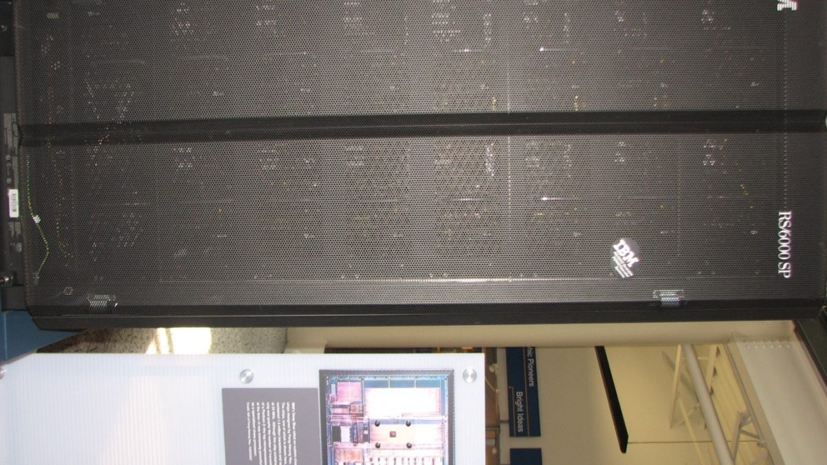
Led by Feng-hsiung Hsu, Murray Campbell, and Joe Hoane, Deep Blue was an engineering marvel combining brute-force parallel hardware with grandmaster heuristics:

• Hardware Muscle: A 32-node IBM RS/6000 SP supercomputer driving 480 custom chess VLSI chips.
• Search Throughput: Evaluated 200 million chess positions per second (compared to Kasparov’s human rate of approximately 2 to 3 positions per second).
• Algorithmic Depth: Executed iterative deepening Alpha-Beta minimax search up to 14 plies (half-moves) deep in normal play, extending to 40 plies in tactical sharp positions via quiescence search and singular extensions.
• Evaluation Function: Over 8,000 hand-tuned evaluation features, including king safety, pawn structure, rook outposts, and a 700,000-position grandmaster opening library combined with Ken Thompson’s 5-piece endgame databases.

May 11, 1997: Game 6

Tied at 2.5 points each after five games, the rubber match of Game 6 ended in sudden, historic shock. Kasparov played the Caro-Kann Defense. Deep Blue countered with an aggressive, intuitive knight sacrifice on move 8 ($8. \text{Nxe6}!$), ripping open Kasparov’s king defenses. Rattled and demoralized, Kasparov made a defensive blunder and resigned in just 19 moves—the shortest defeat of his entire championship career.

Deep Blue did not possess consciousness, intuition, or common sense; it was a pure mathematical calculating engine. Yet by conquering the intellectual summit of human strategic games through raw silicon search and specialized VLSI chips, it irrevocably demonstrated that machines could surpass the greatest minds of humanity in complex intellectual domains.

---