At the computational core of nearly every exponential quantum speedup—from period finding and discrete logarithms to quantum chemistry Hamiltonians—lies the Quantum Fourier Transform (QFT) and its algorithmic sibling, Quantum Phase Estimation (QPE). While classical Fast Fourier Transform (FFT) algorithms require $mathcal{O}(N log N)$ operations over an $N$-element vector, the QFT transforms an $n$-qubit quantum state ($N = 2^n$) in a mere $mathcal{O}(n^2) = mathcal{O}((log N)^2)$ elementary quantum gate operations, achieving an exponential structural compression of frequency space.
1. The Algebraic Mapping: From DFT to QFT
The classical Discrete Fourier Transform (DFT) acts on a complex vector $x = (x_0, x_1, dots, x_{N-1})^T in mathbb{C}^N$ to produce the transformed vector $y = (y_0, y_1, dots, y_{N-1})^T$ according to:
[
y_k = frac{1}{sqrt{N}} sum_{j=0}^{N-1} x_j omega^{j k}, quad text{where } omega = e^{2pi i / N}
]
In quantum mechanics, this linear transformation is elevated to a unitary operator acting on the orthonormal computational basis states ${|0rangle, |1rangle, dots, |N-1rangle}$ of an $n$-qubit Hilbert space $mathcal{H}^{otimes n}$ ($N = 2^n$):
[
text{QFT}_N |jrangle = frac{1}{sqrt{N}} sum_{k=0}^{N-1} e^{2pi i j k / 2^n} |krangle
]
Because the transformation matrix $F_N$ satisfies $F_N^dagger F_N = I_N$, the QFT is strictly unitary. When applied to an arbitrary superposition $|psirangle = sum_{j=0}^{N-1} x_j |jrangle$, the amplitudes transform exactly as the classical DFT coefficients:
[
text{QFT}_N |psirangle = sum_{k=0}^{N-1} y_k |krangle, quad y_k = frac{1}{sqrt{N}} sum_{j=0}^{N-1} x_j e^{2pi i j k / 2^n}
]
2. Product Representation and Circuit Synthesis
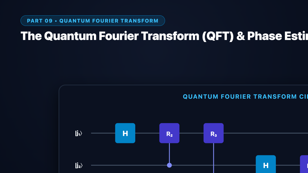
The brilliance of the QFT circuit construction, pioneered by Don Coppersmith, stems from expressing the output state as an unentangled product state. Let $j$ be represented in binary notation as $j = j_1 j_2 dots j_n = sum_{l=1}^n j_l 2^{n-l}$, and denote fractional binary numbers as:
[
0.j_l j_{l+1} dots j_n = sum_{m=l}^n j_m 2^{-(m-l+1)}
]
Expanding the QFT sum into binary components yields the product decomposition:
[
text{QFT}_N |j_1 j_2 dots j_nrangle = frac{1}{sqrt{2^n}} bigotimes_{l=1}^n left( |0rangle + e^{2pi i (0.j_l j_{l+1} dots j_n)} |1rangle right)
]
Notice that each individual output qubit is in a separable state whose phase depends exclusively on the least significant binary digits of the input state. This immediately dictates the circuit topology using two elementary gate families:
- The Single-Qubit Hadamard Gate ($H$): Produces the primary superposition and the most significant fractional phase $0.j_l$:
[
H |j_lrangle = frac{1}{sqrt{2}} left( |0rangle + e^{2pi i (0.j_l)} |1rangle right) = frac{1}{sqrt{2}} left( |0rangle + (-1)^{j_l} |1rangle right)
] - Controlled Phase-Shift Gates ($R_k$): Adds the finer fractional phases conditioned on target control qubits:
[
R_k = begin{pmatrix} 1 & 0 \ 0 & e^{2pi i / 2^k} end{pmatrix}
]
For an $n$-qubit register:
- Qubit 1 undergoes $1$ Hadamard and $n-1$ controlled phase rotations ($R_2, R_3, dots, R_n$).
- Qubit 2 undergoes $1$ Hadamard and $n-2$ controlled rotations ($R_2, dots, R_{n-1}$).
- Continuing inductively, the total number of two-qubit controlled phase gates is:
[
sum_{m=1}^{n-1} m = frac{n(n-1)}{2}
] - Adding $n$ Hadamard gates and $lfloor n/2 rfloor$ SWAP gates to reverse the bit order results in a total gate complexity of:
[
text{Total Gates} = frac{n(n-1)}{2} + n + lfloor n/2 rfloor = mathcal{O}(n^2)
]
For $N = 2^{64}$ ($n = 64$ qubits), a classical FFT requires $approx 64 times 2^{64} approx 1.18 times 10^{21}$ operations, whereas the QFT circuit requires merely $approx 2,080$ quantum gates.
3. Quantum Phase Estimation (QPE)
While QFT cannot be used to directly read out the classical Fourier coefficients (as quantum measurement collapses the state), its profound power emerges when run in reverse ($text{QFT}^dagger$) inside the Quantum Phase Estimation protocol.
Given a unitary operator $U$ and an eigenvector $|urangle$ satisfying:
[
U |urangle = e^{2pi i theta} |urangle, quad theta in [0, 1)
]
QPE extracts an $n$-bit binary estimate of the unknown phase $theta = 0.theta_1 theta_2 dots theta_n$. The circuit operates across two registers:
- Counting Register (Register 1): $t$ qubits initialized to $|0rangle^{otimes t}$, which will record the binary representation of $theta$.
- Target Register (Register 2): Contains the eigenvector $|urangle$.
The Algorithmic Stages of QPE:
- Superposition Initialization: Apply $H^{otimes t}$ to Register 1:
[
|psi_0rangle = frac{1}{sqrt{2^t}} sum_{j=0}^{2^t-1} |jrangle |urangle
] - Controlled-Unitary Cascade ($C-U^{2^k}$): Apply controlled-$U^{2^k}$ operations from the $k$-th qubit of Register 1 onto Register 2. Because $U^{2^k} |urangle = e^{2pi i 2^k theta} |urangle$, the phase kicks back into Register 1:
[
|psi_1rangle = frac{1}{sqrt{2^t}} sum_{j=0}^{2^t-1} e^{2pi i theta j} |jrangle |urangle
] - Inverse Quantum Fourier Transform ($text{QFT}^dagger$): Apply $text{QFT}^dagger$ to Register 1. Notice that $|psi_1rangle$ is precisely the QFT of the state $|2^t thetarangle$. Thus:
[
text{QFT}^dagger left( frac{1}{sqrt{2^t}} sum_{j=0}^{2^t-1} e^{2pi i theta j} |jrangle right) = |2^t thetarangle = |theta_1 theta_2 dots theta_trangle
] - Computational Basis Measurement: Measuring Register 1 yields the exact digits of $theta$ with probability $1$ if $theta$ can be expressed as a $t$-bit binary fraction.
4. Precision, Error Bounds & Success Probability
If $theta$ cannot be represented exactly with $t$ bits, QPE rounds to the closest dyadic rational $b/2^t$. To guarantee an estimate accurate to $n$ bits with success probability at least $1 – epsilon$, the required number of evaluation qubits $t$ must satisfy:
[
t = n + leftlceil log_2 left( 2 + frac{1}{2epsilon} right) rightrceil
]
The probability $P(m)$ of measuring a state $m$ close to $2^t theta$ is governed by Fejér-type interference kernel:
[
P(m) = frac{1}{2^{2t}} left| frac{1 – e^{2pi i (2^t theta – m)}}{1 – e^{2pi i (2^t theta – m)/2^t}} right|^2 = frac{1}{2^{2t}} frac{sin^2(pi(2^t theta – m))}{sin^2(pi(2^t theta – m)/2^t)}
]
QPE serves as the master subroutine for Shor’s factoring algorithm, the HHL algorithm for linear systems, Hamiltonian simulation, and quantum ground state preparation.