Quantum Information & Quantum Computing (Part 19): Quantum Simulation, The Feynman Thesis & The Variational Quantum Eigensolver (VQE)

In May 1982, Richard Feynman delivered a keynote address at MIT titled “Simulating Physics with Computers,” in which he pronounced the founding charter of quantum computation: “Nature isn’t classical, dammit, and if you want to make a simulation of nature, you’d better make it quantum mechanical!” Because simulating an $N$-electron molecule classically requires storing a state vector of dimension $2^N$—demanding more memory than the total number of atoms in the observable universe for just a few hundred electrons—quantum simulation represents the most direct, transformative application of quantum computers to chemistry, materials science, and drug discovery.

1. Mapping Fermions to Qubits: The Jordan-Wigner Transformation

Molecular electronic structures are governed by fermionic electrons obeying anti-commutation relations ${c_i, c_j^dagger} = delta_{ij}$. Qubits, however, are distinguished spin-1/2 systems whose Pauli operators commute at different sites $[X_i, X_j] = 0$ ($i neq j$).

The Jordan-Wigner Transformation maps fermionic creation and annihilation operators to multi-qubit Pauli spin operators while strictly preserving anti-commutation through non-local Pauli $Z$ strings:

[
c_j^dagger = left( bigotimes_{k=1}^{j-1} Z_k right) otimes sigma_j^-, quad c_j = left( bigotimes_{k=1}^{j-1} Z_k right) otimes sigma_j^+
]

where $sigma_j^pm = frac{1}{2}(X_j mp i Y_j)$. The electronic molecular Hamiltonian:

[
H = sum_{pq} h_{pq} c_p^dagger c_q + frac{1}{2} sum_{pqrs} h_{pqrs} c_p^dagger c_q^dagger c_s c_r
]

is thereby compiled into a linear combination of Pauli string operators acting on the quantum processor:

[
H = sum_k c_k P_k, quad P_k in {I, X, Y, Z}^{otimes n}
]

2. Hamiltonian Simulation via Trotter-Suzuki Decomposition

To simulate the time evolution operator $U(t) = e^{-iHt}$, we must exponentiate a Hamiltonian composed of non-commuting terms $H = sum_{j=1}^m H_j$ ($[H_j, H_k] neq 0$). The Baker-Campbell-Hausdorff (BCH) theorem forbids simple product factorization. Instead, we employ the Lie-Trotter-Suzuki Product Formulas:

[
e^{-iHt} = lim_{r to infty} left( prod_{j=1}^m e^{-i H_j t / r} right)^r
]

For a finite Trotter step count $r$, the second-order symmetric Suzuki-Trotter formula suppresses algorithmic discretization error to:

[
S_2(tau) = prod_{j=1}^m e^{-i H_j tau / 2} prod_{j=m}^1 e^{-i H_j tau / 2} = e^{-i H tau} + mathcal{O}(tau^3)
]

By executing these discrete gate slices, the quantum processor tracks the continuous time-dependent Schrödinger evolution with polynomial resource overhead.

3. The Variational Quantum Eigensolver (VQE)

While Trotterized simulation requires deep, coherent quantum circuits that exceed the coherence times of contemporary Noisy Intermediate-Scale Quantum (NISQ) devices, the Variational Quantum Eigensolver (VQE) (Peruzzo et al., 2014) provides a hybrid quantum-classical alternative.

The Rayleigh-Ritz Variational Principle

VQE seeks the ground state energy $E_0$ of a molecular Hamiltonian $H$. The Rayleigh-Ritz variational theorem states that for any normalized trial state $|psi(vec{theta})rangle$ parameterized by classical angles $vec{theta} = (theta_1, dots, theta_p)$:

[
langle H rangle_{vec{theta}} = frac{langle psi(vec{theta}) | H | psi(vec{theta}) rangle}{langle psi(vec{theta}) | psi(vec{theta}) rangle} ge E_0
]

Equality holds if and only if $|psi(vec{theta})rangle$ is the exact ground state eigenvector.

The Hybrid Optimization Loop:

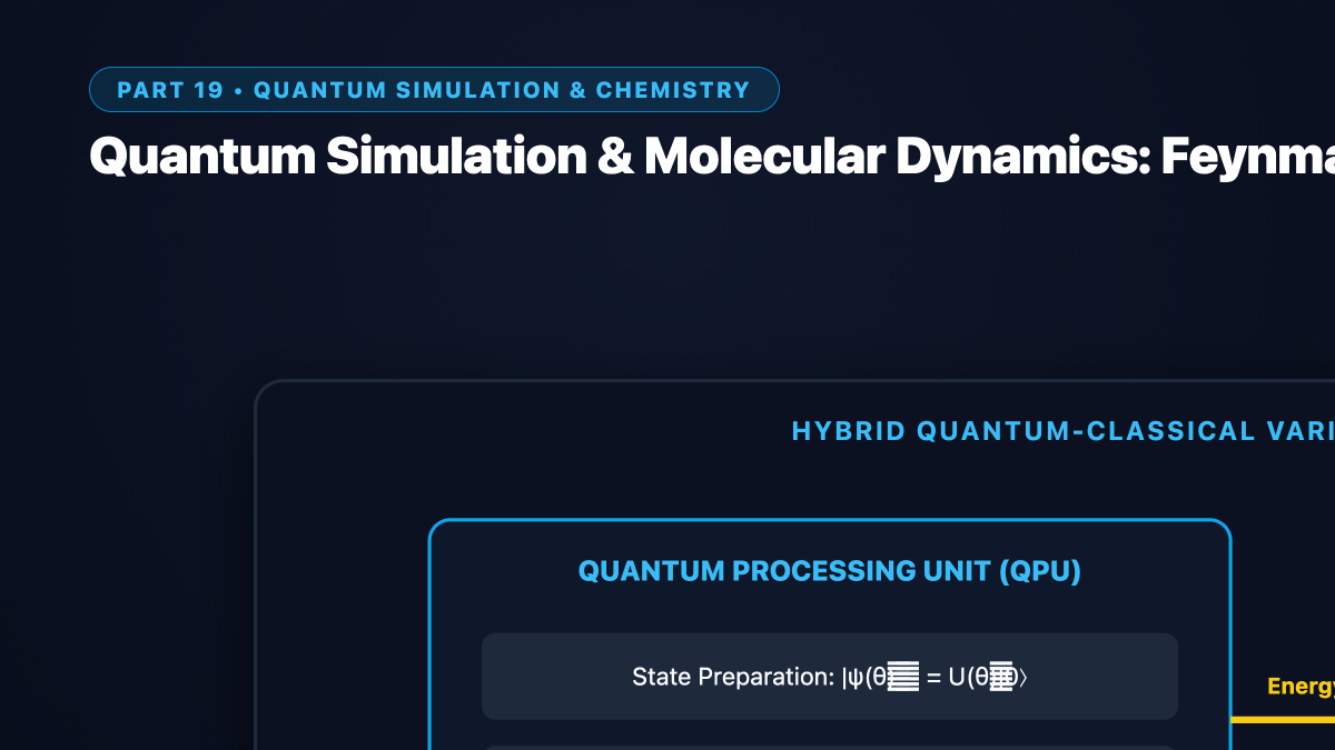
1. Quantum Processing Unit (QPU):
   • Prepares the parameterized ansatz state $|psi(vec{theta})rangle = U(vec{theta}) |0rangle^{otimes n}$ (e.g., Unitary Coupled Cluster UCCSD or Hardware-Efficient Ansatz).
   • Measures the expectation values of each Pauli string term $langle P_k rangle = langle psi(vec{theta}) | P_k | psi(vec{theta}) rangle$.
   • Computes the total energy expectation $langle H rangle_{vec{theta}} = sum_k c_k langle P_k rangle$.
2. Classical Optimization Engine:
   • Receives $langle H rangle_{vec{theta}}$ and computes gradient vectors $nabla_{vec{theta}} langle H rangle$ using the exact quantum Parameter-Shift Rule:
     [
     frac{partial langle H rangle}{partial theta_j} = frac{langle H rangle_{vec{theta} + frac{pi}{2} hat{e}_j} – langle H rangle_{vec{theta} – frac{pi}{2} hat{e}_j}}{2}
     ]
   • Updates the parameters using classical optimizers (BFGS, COBYLA, or Adam): $vec{theta}_{t+1} = vec{theta}_t – eta nabla langle H rangle$.
3. The loop iterates until convergence to the ground state energy $E_0$.

Shakil Mahmud Shazal

Senior Software Engineer based in Dhaka, Bangladesh. Building scalable web architectures and writing at the intersection of computer science, physical systems, history, and ideas.