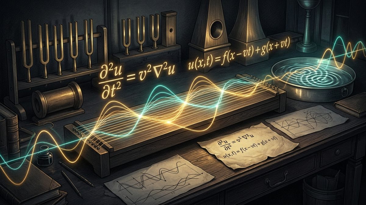
Pluck the string of a violin or harp. A shimmering blur sweeps back and forth across the taut gut, sending invisible ripples of compression through the air that strike your ear as a crystalline musical note. In 1746, the French polymath Jean le Rond d’Alembert asked a deceptively simple question: What is the exact mathematical law governing that vibrating string? His answer gave birth to the very first partial differential equation in human history: The Wave Equation. From violin chords and ocean tsunamis to seismic earthquakes, fiber-optic light, and the quantum wavefunctions of matter, the universe vibrates to d’Alembert’s rhythm.
1. The Formula: Curvature in Time Equals Curvature in Space
In one spatial dimension, the classical wave equation relates the second time derivative of a displacement field $u(x, t)$ to its second spatial derivative:
In three spatial dimensions, the spatial derivative generalizes into the Laplacian operator $nabla^2 = frac{partial^2}{partial x^2} + frac{partial^2}{partial y^2} + frac{partial^2}{partial z^2}$:
This compact relation expresses an astonishing physical principle: temporal acceleration is directly proportional to spatial curvature.
- $u(mathbf{x}, t)$ (The Displacement Field): The amplitude of the disturbance at spatial point $mathbf{x}$ and time $t$. For a string, it is transverse displacement; for sound, acoustic pressure deviation $Delta p$; for light, electric and magnetic field amplitudes $mathbf{E}$ and $mathbf{B}$.
- $frac{partial^2 u}{partial t^2}$ (Temporal Acceleration): How quickly the local speed of oscillation changes with time.
- $nabla^2 u$ (Spatial Curvature / Laplacian): Measures whether a point is higher or lower than the average of its immediate neighbors. If a point on a string is at a sharp peak, the surrounding points are lower; the spatial curvature is negative, generating a downward restoring acceleration.
- $v$ (Wave Propagation Velocity): The finite speed at which disturbances travel through the medium: $v = sqrt{T/mu}$ for a string under tension $T$ with linear mass density $mu$.
2. First-Principles Derivation from Newton’s Second Law
To see how d’Alembert arrived at this relation, consider an infinitesimal segment of a taut string between $x$ and $x + dx$, with uniform linear mass density $mu$ and constant tension $T$. The mass of this microscopic slice is $dm = mu , dx$.
At the left end $x$, tension pulls downward along the tangent angle $theta_1$. At the right end $x + dx$, tension pulls upward along $theta_2$. For small amplitudes, the vertical components of tension are:
The net vertical restoring force $dF_y$ acting on the string element is the difference between these two boundary pulls:
By Newton’s second law, net force equals mass times vertical acceleration ($dF_y = dm cdot a_y = (mu , dx) frac{partial^2 u}{partial t^2}$):
Dividing through by the infinitesimal element $dx$ and defining the phase velocity $v = sqrt{T/mu}$, we obtain d’Alembert’s one-dimensional wave equation:
3. D’Alembert’s Traveling Wave Solution
How does one solve this partial differential equation? D’Alembert introduced a brilliant change of characteristic coordinates that factorizes the wave operator:
Applying the multi-variable chain rule transforms the wave equation into the trivial hyperbolic form:
Integrating with respect to $xi$ and $eta$ immediately yields the general solution:
This solution carries profound physical meaning: any disturbance can be decomposed into two independent, rigid waveforms. The function $f(x – vt)$ represents an arbitrary profile traveling forward to the right at constant velocity $v$ without changing shape; $g(x + vt)$ represents a profile traveling backward to the left at velocity $v$. When these traveling waves reflect off fixed boundaries (such as the nut and bridge of a guitar), they interfere constructively to create standing harmonic modes:
4. The Bridge to Maxwell, Optics, and Quantum Mechanics
- Electromagnetic Waves: In 1865, James Clerk Maxwell took the curl of his electromagnetic equations in free space and discovered that electric and magnetic fields satisfy d’Alembert’s 3D wave equation: $nabla^2 mathbf{E} = mu_0 varepsilon_0 frac{partial^2 mathbf{E}}{partial t^2}$. The speed of these waves $c = 1/sqrt{mu_0 varepsilon_0} approx 3 times 10^8 text{ m/s}$ matched the measured speed of light, uniting electricity, magnetism, and optics in a single stroke.
- Seismology: Earthquakes propagate through the Earth’s crust as primary compressional waves (P-waves: $v_p = sqrt{frac{K + frac{4}{3}mu}{rho}}$) and secondary shear waves (S-waves: $v_s = sqrt{mu/rho}$), enabling geophysicists to map the liquid outer core of our planet.
- Quantum Mechanics: Erwin Schrödinger’s 1926 wave equation $ihbar frac{partial psi}{partial t} = -frac{hbar^2}{2m}nabla^2psi$ is the quantum descendant of d’Alembert’s classical wave dynamics, describing the probability amplitude waves of atomic matter.




