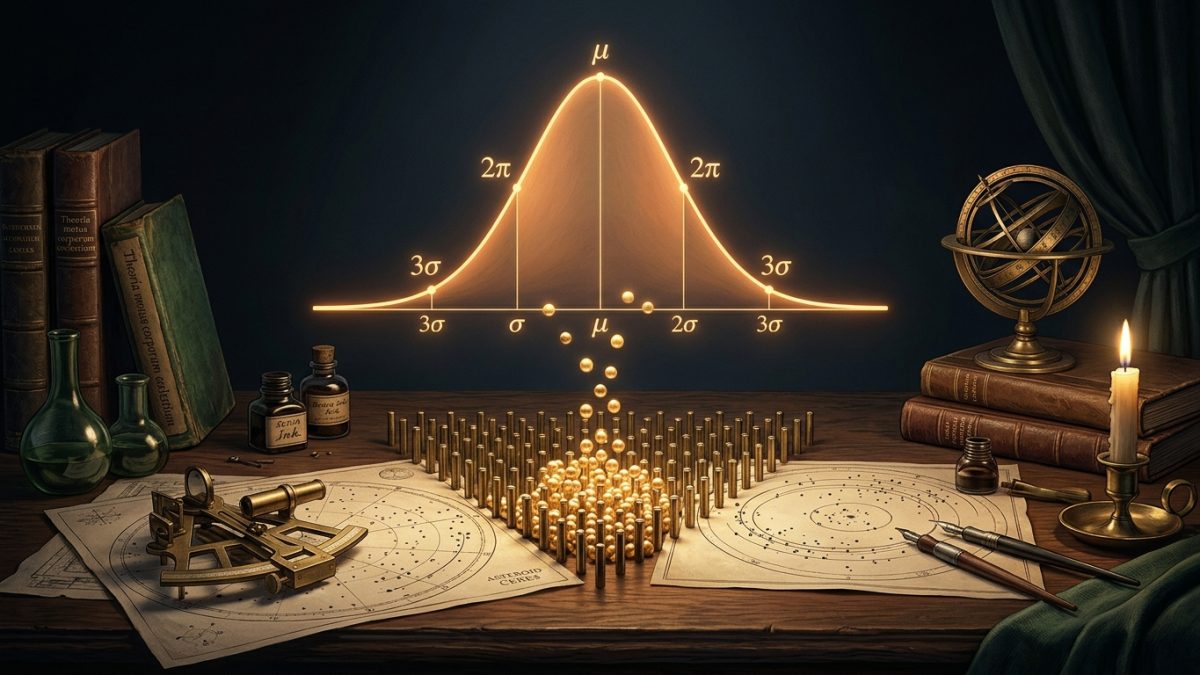
On New Year’s Day in 1801, Italian astronomer Giuseppe Piazzi glimpsed a faint, wandering pinpoint of light in the constellation Taurus. It was Ceres, the first discovered asteroid. Forty days later, Ceres vanished behind the blinding glare of the Sun. Astronomers were desolate: tracking an uncharted celestial body from sparse, imprecise telescope measurements seemed mathematically impossible. Enter twenty-four-year-old Carl Friedrich Gauss. Armed with a revolutionary theory of observational errors and a mathematical bell-shaped curve, Gauss calculated Ceres’s trajectory so precisely that astronomers pointed their telescopes back into the night sky months later and found the lost planetoid within one degree of his prediction. The mathematical engine powering Gauss’s triumph was the Normal Distribution: the universal law governing randomness, measurement uncertainty, and collective order.
1. The Formula: The Anatomy of the Bell Curve
The probability density function (PDF) of a normal or Gaussian random variable $X sim mathcal{N}(mu, sigma^2)$ is defined across the entire real continuum $(-infty, infty)$ by the immortal equation:
Every single parameter and constant in this expression tells a profound story of geometry, probability, and calculus:
- $x$ (The Continuous Variable): The observed measurement, deviation, or experimental value on the real number axis.
- $mu$ (The Mean / Location Parameter): The expected value or center of mass ($mathbb{E}[X] = mu$). The peak of the symmetric bell curve occurs exactly at $x = mu$, where the first derivative vanishes: $f'(mu) = 0$.
- $sigma$ (Standard Deviation / Scale Parameter): The characteristic width of dispersion. The inflection points of the curve—where concavity shifts from downward to upward—occur precisely at $x = mu pm sigma$, where the second derivative equals zero: $f”(mu pm sigma) = 0$.
- The Exponential Core $expleft(-frac{(x-mu)^2}{2sigma^2}right)$:: Governs how probabilities decay. Unlike linear or polynomial decay, the squared deviation $(x-mu)^2$ in the exponent ensures that extreme outliers become exponentially and super-exponentially improbable.
- The Normalizing Factor $frac{1}{sigmasqrt{2pi}}$: Ensures that the total integrated probability over all conceivable outcomes equals unity: $int_{-infty}^infty f(x) , dx = 1$. The emergence of the geometric circle constant $pi$ inside a pure probability distribution reflects the deep Euclidean symmetry of two-dimensional rotational space.
2. The Gaussian Integral: Why Does $pi$ Appear in Probability?
One of the most awe-inspiring questions in analysis is why $pi$—the ratio of a circle’s circumference to its diameter—resides in a formula describing human heights, stellar errors, and particle velocities. The answer lies in the classical double integral evaluation developed by Siméon Denis Poisson.
Consider the fundamental Gaussian integral $I = int_{-infty}^infty e^{-x^2} dx$. The function $e^{-x^2}$ has no elementary antiderivative in terms of standard algebraic or trigonometric functions. To compute it, we square the integral and evaluate it over the two-dimensional Cartesian plane:
Because the integrand $e^{-(x^2 + y^2)} = e^{-r^2}$ is radially symmetric, we transform the coordinates from Cartesian $(x,y)$ to polar $(r, theta)$, where $x^2 + y^2 = r^2$ and the area element is $dx , dy = r , dr , dtheta$:
The angular integral simply evaluates to the full circle sweep: $int_0^{2pi} dtheta = 2pi$. The radial integral is directly solvable by the substitution $u = r^2$, giving $du = 2r , dr$:
Multiplying these factors yields $I^2 = 2pi cdot frac{1}{2} = pi$, which immediately proves:
Applying the change of variables $z = frac{x – mu}{sqrt{2}sigma}$ gives $dx = sqrt{2}sigma , dz$, directly verifying the normalization factor $frac{1}{sigmasqrt{2pi}}$. Circular symmetry in two independent random error dimensions is the geometric reason $pi$ governs Gaussian probability.
3. The Central Limit Theorem: Order from Microscopic Chaos
Why is the normal distribution ubiquitous in nature? The answer is the Central Limit Theorem (CLT), mathematically formalized by Pierre-Simon Laplace in 1810 and later generalized by Aleksandr Lyapunov and Jarl Waldemar Lindeberg.
The Central Limit Theorem asserts that if you collect a large sequence of independent and identically distributed (i.i.d.) random variables $X_1, X_2, dots, X_n$ with an arbitrary probability distribution—whether uniform, skewed, bimodal, or discrete—possessing a finite mean $mu$ and finite variance $sigma^2$, their standardized sample mean converges in distribution to the standard normal distribution as $n to infty$:
This is nature’s grand statistical attractor. Whenever an observed macroscopic phenomenon—such as the flight of a pollen grain, the voltage fluctuation across a resistor, or the height of an organism—is the cumulative result of thousands of tiny, independent microscopic nudges, the individual distributions wash out completely. What remains is the universal bell curve.
4. Scientific and Modern Computational Impact
- Statistical Mechanics: James Clerk Maxwell used the Gaussian error distribution in 1860 to derive the speed distribution of molecules in an ideal gas: $f(v) propto v^2 expleft(-frac{mv^2}{2k_B T}right)$. The temperature of a gas is fundamentally the variance of its microscopic Gaussian velocity fluctuations.
- Machine Learning and Deep Learning: In artificial neural networks, weight matrices are initialized using Gaussian distributions (e.g., He or Xavier/Glorot initialization: $W sim mathcal{N}left(0, sqrt{2/n_{text{in}}}right)$) to prevent exploding or vanishing gradients during backpropagation.
- Quantitative Finance: The Black-Scholes-Merton option pricing formula calculates derivative values under the assumption that asset returns follow a log-normal random walk driven by Gaussian Brownian motion.
- Signal Processing & Telecommunications: Additive White Gaussian Noise (AWGN) is the universal baseline model for channel noise in 5G, Wi-Fi, optical fiber, and deep-space telemetry.
5. Bilingual Mathematical Reference Table
| English Term | বাংলা পরিভাষা | Mathematical Symbol / Role |
|---|---|---|
| Normal / Gaussian Distribution | পরিমিত / গাউসীয় বিন্যাস | $X sim mathcal{N}(mu, sigma^2)$ |
| Probability Density Function (PDF) | সম্ভাব্যতা ঘনত্ব অপেক্ষক | $f(x) ge 0, int f(x)dx = 1$ |
| Expected Value / Mean | প্রত্যাশিত মান / গড় | $mathbb{E}[X] = mu$ |
| Standard Deviation / Variance | পরিমিত ব্যবধান / ভেদমান | $sigma = sqrt{text{Var}(X)}$ |
| Inflection Point | অনতিবিন্দু / বক্রতা বদল বিন্দু | $x = mu pm sigma$ |
| Central Limit Theorem | কেন্দ্রীয় সীমা উপপাদ্য | $sqrt{n}(bar{X}_n – mu) xrightarrow{d} mathcal{N}(0, sigma^2)$ |
| Gaussian Integral | গাউসীয় সমাকলন | $int_{-infty}^infty e^{-x^2}dx = sqrt{pi}$ |
| Brownian Motion / Random Walk | ব্রাউনীয় গতি / দ্বৈব চলন | $B(t) sim mathcal{N}(0, t)$ |




