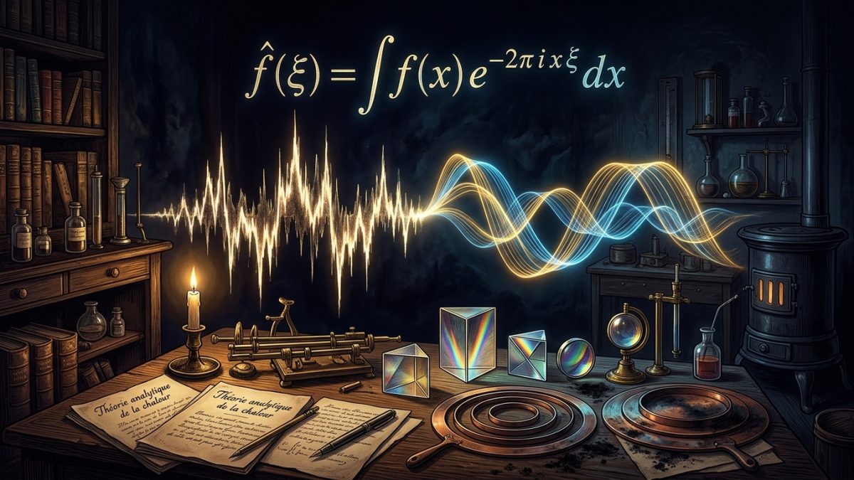
In 1807, a French mathematician and imperial prefect named Jean-Baptiste Joseph Fourier walked into the Académie des Sciences in Paris with a manuscript that seemed like pure heresy. He claimed that any mathematical function—no matter how jagged, discontinuous, or broken—could be recreated perfectly as an infinite sum of smooth sine and cosine waves. The greatest mathematicians of the era, including Joseph-Louis Lagrange and Pierre-Simon Laplace, rejected his paper, arguing that continuous trigonometric functions could never construct a square corner. But Fourier was right, and the establishment was wrong. Today, the Fourier Transform is the mathematical foundation of the digital universe: without it, there would be no MP3 audio, no JPEG images, no MRI scanners, no 5G cellular networks, and no modern quantum spectroscopy.
1. The Formula: From Time Domain to Frequency Spectrum
The continuous Fourier Transform translates a function $f(t)$ from the time or spatial domain into its frequency-domain spectrum $hat{f}(xi)$:
And remarkably, the original signal can be reconstructed without losing a single bit of information via the Inverse Fourier Transform:
The mathematical architecture of this transform is breathtaking in its elegance:
- $f(t)$ (The Temporal or Spatial Signal): The observed waveform, audio pressure signal, or spatial image intensity evolving across time $t$.
- $xi$ (Frequency): Measured in cycles per second (Hertz, $text{Hz}$), representing the oscillation rate of individual constituent waves. In angular frequency notation ($omega = 2pixi$), the transform is written $hat{f}(omega) = int_{-infty}^infty f(t) e^{-iomega t} dt$.
- $e^{-2pi i xi t}$ (The Complex Exponential Kernel): By Euler’s formula, $e^{-2pi i xi t} = cos(2pi xi t) – i sin(2pi xi t)$. This kernel wraps the input signal $f(t)$ around the complex unit circle at an angular frequency of $xi$ cycles per second.
- $hat{f}(xi)$ (The Complex Spectral Amplitude): A complex number whose magnitude $|hat{f}(xi)|$ gives the strength of frequency $xi$ in the signal, and whose argument $arg(hat{f}(xi))$ gives its phase alignment. When frequency $xi$ resonates with an intrinsic frequency of $f(t)$, the wrapped circle points cluster on one side, causing the integrated center of mass $hat{f}(xi)$ to spike dramatically.
2. Mathematical Properties: Duality, Convolution, and Energy
The Fourier transform possesses deep structural symmetries that convert intractable calculus operations into elementary algebra:
- Differentiation Becomes Multiplication: Taking the derivative of a signal in time corresponds to simply multiplying its spectrum by frequency: $$mathcal{F}left{ frac{df}{dt} right} = (2pi i xi) , hat{f}(xi)$$ This algebraic transformation is why partial differential equations governing heat, diffusion, and electrodynamics can be solved in closed form.
- The Convolution Theorem: The complex temporal convolution of two signals $(f * g)(t) = int_{-infty}^infty f(tau) g(t – tau) dtau$ maps directly to elementary pointwise multiplication in the frequency domain: $$mathcal{F}{ f * g } = hat{f}(xi) cdot hat{g}(xi)$$ This single theorem underpins modern digital filtering, audio reverb synthesis, and image blurring/sharpening algorithms.
- Plancherel / Parseval Energy Conservation: The total energy of a signal measured in the time domain is strictly equal to the total energy distributed across its frequency spectrum: $$int_{-infty}^infty |f(t)|^2 , dt = int_{-infty}^infty |hat{f}(xi)|^2 , dxi$$
3. The Uncertainty Principle of Signals and Quanta
Can a musical note be both infinitely short in duration and possess an infinitely precise musical pitch? The Fourier Transform gives a rigorous, negative answer. A signal sharply localized in time (like a sharp gunshot click, approaching a Dirac delta function $delta(t)$) spreads out across all frequencies equally ($hat{f}(xi) = 1$). Conversely, an eternal pure sinusoidal note contains exactly one frequency, but extends over all time from $-infty$ to $+infty$.
Mathematically, if we define the temporal variance $sigma_t^2 = int t^2 |f(t)|^2 dt$ and frequency variance $sigma_xi^2 = int xi^2 |hat{f}(xi)|^2 dxi$, the Fourier Transform enforces the fundamental inequality:
When Werner Heisenberg formulated the Quantum Uncertainty Principle in 1927 ($Delta x cdot Delta p ge frac{hbar}{2}$), he was not uncovering an arbitrary restriction of measurement instruments; he was observing the Fourier Transform operating directly on quantum matter waves, where position $psi(x)$ and momentum $phi(p)$ are exact Fourier dual pairs.
4. The Fast Fourier Transform (FFT): The Algorithm of Civilization
Calculating the discrete Fourier transform of a sequence of $N$ data points naively requires $O(N^2)$ operations. For a 4K video frame or high-resolution audio file with $N = 10^6$ samples, $10^{12}$ operations per frame would grind computers to a halt. In 1965, J. W. Cooley and John Tukey rediscovered the Fast Fourier Transform (FFT) algorithm (originally sketched in unpublished notes by Gauss in 1805). By recursively dividing the transform into even and odd components, FFT reduced computational complexity from $O(N^2)$ to $O(N log_2 N)$.
This exponential leap in efficiency made real-time digital signal processing possible. Every time you stream Spotify music, conduct a video call over Wi-Fi, view a JPEG photo, or undergo an MRI scan, billions of Cooley-Tukey butterfly operations decompose reality into Fourier harmonics.




