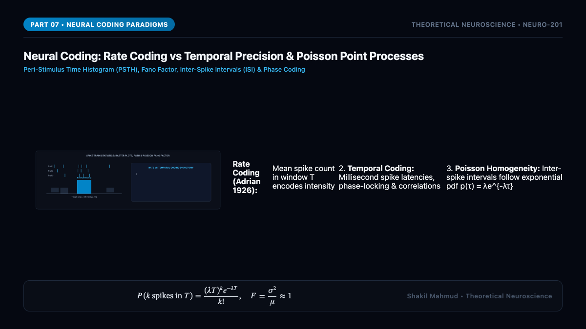
Because action potentials are stereotypic all-or-none events, an individual spike carries no information in its amplitude or waveform. The information that sculpts conscious experience is encoded purely in the temporal arrangement of identical electrical impulses: the Neural Code. For nearly a century, theoretical neuroscience has debated whether the brain represents reality via the slow average frequency of spikes (Rate Coding) or through the millisecond precision and rhythmic phase of individual discharges (Temporal Coding).
1. Adrian’s Rate Coding & Firing Rate Functions
In 1926, Edgar Adrian recorded sensory fibers in frog muscle stretch receptors and discovered that stronger physical stretching did not increase spike height, but increased the frequency of spikes fired per unit time. This gave birth to Rate Coding.
Formally, given a spike train represented as a sequence of Dirac delta functions $rho(t) = sum_{i=1}^n delta(t – t_i)$, the instantaneous firing rate $r(t)$ is estimated across repeated trials by the Peri-Stimulus Time Histogram (PSTH) or continuous Gaussian kernel convolution:
r(t) = frac{1}{Delta t} frac{1}{K} sum_{k=1}^K N_k(t, t + Delta t) approx int_{-infty}^infty w(tau) rho(t – tau) dtau
While rate coding accounts well for peripheral motor drives and slow sensory adaptation, it fails to explain ultra-fast sensory perception (e.g., humans recognizing complex natural images within $100text{–}150text{ ms}$, where each cortical visual layer has time to fire at most one or two spikes).
2. Temporal Precision & Phase Coding
In contrast to average rates, Temporal Coding posits that precise spike timing carries distinct information unreachable by mean counts:
- Time-to-First-Spike (Latency Coding): Information is encoded in the latency between stimulus onset and the first action potential, enabling sub-millisecond classification.
- Inter-Spike Interval (ISI) Coding: Information resides in higher-order temporal patterns and rhythms within the spike sequence.
- Phase of Firing: In the hippocampus, place cells fire at progressively earlier phases of the ongoing local $4text{–}8text{ Hz}$ extracellular theta oscillation as the animal traverses a place field—a phenomenon known as Phase Precession, where phase carries precise sub-centimeter position data orthogonal to firing rate.
3. Stochastic Spike Statistics: The Homogeneous Poisson Process
In vivo recordings in the awake cerebral cortex reveal remarkable variability: repeated presentations of an identical stimulus yield wildly variable spike counts and timings. To model this, cortical neurons are treated as Point Processes, most commonly the Homogeneous Poisson Process.
Under the Poisson assumption, the probability of observing exactly $k$ spikes within an observation window $T$ given an average rate $lambda$ is governed by the Poisson distribution:
P(k text{ spikes in } T) = frac{(lambda T)^k e^{-lambda T}}{k!}
The time interval $tau$ between consecutive spikes (the Inter-Spike Interval, ISI) is a continuous random variable distributed according to an exponential probability density function:
p(tau) = lambda e^{-lambda tau} quad (tau ge 0)
The mean and variance of the exponential distribution are $langle tau rangle = 1/lambda$ and $text{Var}(tau) = 1/lambda^2$, yielding a Coefficient of Variation of unity: $CV_{text{ISI}} equiv sigma / mu = 1$.
4. The Fano Factor & Inhomogeneous Processes
To quantify neural noise and spike count trial-to-trial variability across repeated presentations, neuroscientists calculate the Fano Factor $F$:
F equiv frac{text{Var}(N_T)}{langle N_T rangle}
For a pure Poisson process, $F = 1.0$. Remarkably, cortical neurons recorded in awake behaving primates exhibit Fano factors ranging between $1.0$ and $1.5$, indicating Poisson-like stochasticity. However, upon the sudden presentation of an attended stimulus or motor execution, Mark Churchland et al. (2010) demonstrated that cortical variability drops systematically ($F to 0.5text{–}0.7$), signaling a transition from unconstrained spontaneous fluctuations to stabilized low-dimensional attractor trajectories.




