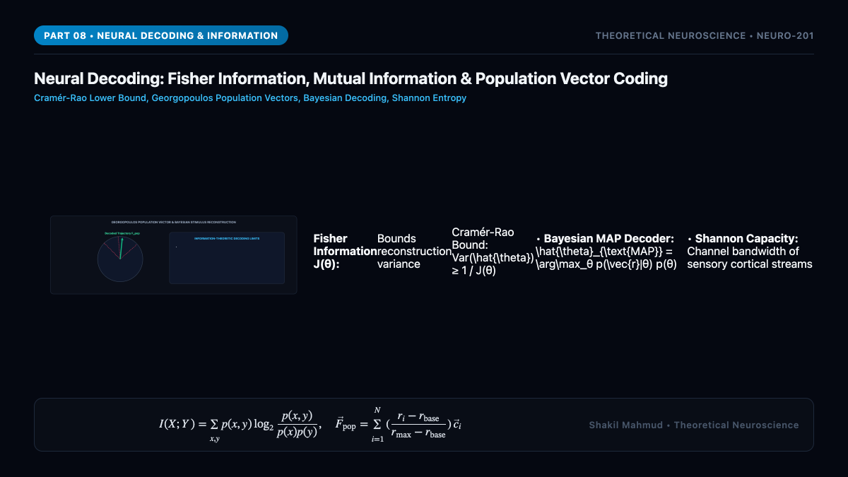
While neural encoding asks how an external physical stimulus produces a pattern of spikes ($p(mathbf{r} | s)$), neural decoding asks the inverse problem faced by downstream brain areas and Brain-Computer Interfaces (BCIs): given an observed spike train $mathbf{r}$, what was the external stimulus $s$? By fusing Claude Shannon’s Information Theory with Ronald Fisher’s estimation theory, modern computational neuroscience mathematically quantifies the channel capacity of sensory cortex and reconstructs intended movements through Population Vector Decoding.
1. Tuning Curves & The Georgopoulos Population Vector
In sensory and motor cortices, individual neurons exhibit broad, smooth bell-shaped Tuning Curves. In 1982, Apostolos Georgopoulos recorded from the primary motor cortex (M1) of rhesus monkeys during 3D arm-reaching tasks, discovering that each neuron fires maximally for a preferred directional vector $vec{c}_i$, decaying as a cosine of angle $theta$:
f_i(theta) = b_i + k_i cos(theta – theta_i) = b_i + vec{k}_i cdot vec{u}
Because an individual neuron’s response is ambiguous (a firing rate of $20text{ Hz}$ could correspond to two different directions symmetrically flanking the preferred direction), the brain decodes direction through an ensemble vote: The Georgopoulos Population Vector $vec{F}_{text{pop}}$:
vec{F}_{text{pop}} = sum_{i=1}^N left( frac{r_i – b_i}{k_i} right) vec{c}_i
Each neuron contributes a vector pointing along its preferred direction $vec{c}_i$, weighted by its baseline-subtracted normalized firing rate. The resulting population vector points with astounding accuracy along the monkey’s actual physical hand trajectory hundreds of milliseconds before movement occurs, forming the algorithmic cornerstone of modern neural prosthetics and BCI implants.
2. Bayesian Decoding: Maximum Likelihood & MAP
Formally, optimal decoding is an exercise in statistical inference. By Bayes’ Rule, the posterior probability of stimulus $s$ given observed spike population vector $vec{r}$ is:
p(s | vec{r}) = frac{p(vec{r} | s) p(s)}{p(vec{r})} propto p(vec{r} | s) p(s)
Assuming conditionally independent Poisson neurons ($p(vec{r} | s) = prod_{i=1}^N frac{f_i(s)^{r_i} e^{-f_i(s)}}{r_i!}$), the log-likelihood is:
ln p(vec{r} | s) = sum_{i=1}^N r_i ln f_i(s) – sum_{i=1}^N f_i(s) + text{const}
The Maximum Likelihood Estimator (MLE) $hat{s}_{text{ML}} = argmax_s ln p(vec{r} | s)$ maximizes the likelihood of the neural response. When prior behavioral context $p(s)$ is available, the Maximum A Posteriori (MAP) estimator $hat{s}_{text{MAP}} = argmax_s [ln p(vec{r} | s) + ln p(s)]$ provides the Bayesian optimal perceptual estimate, elegantly explaining sensory visual illusions as optimal Bayesian compromises between noisy sensory evidence and natural world priors.
3. Fisher Information & The Cramér-Rao Lower Bound
How accurately can a population of neurons possibly encode a continuous stimulus parameter $s$? The ultimate physical limit on decoding precision is dictated by Fisher Information $J(s)$:
J(s) equiv mathbb{E}_{vec{r}|s} left[ left( frac{partial ln p(vec{r}|s)}{partial s} right)^2 right] = sum_{i=1}^N frac{(f_i'(s))^2}{f_i(s)}
By the Cramér-Rao Inequality, the variance of any unbiased estimator $hat{s}(vec{r})$ is strictly bounded from below by the reciprocal of the Fisher information:
text{Var}(hat{s}) ge frac{1}{J(s)}
Notice that $J(s)$ depends on $(f_i'(s))^2$, the square of the derivative of the tuning curve. Therefore, the neurons that provide the greatest discriminatory information about a stimulus are not those firing at their peak (where $f'(s) approx 0$), but those whose tuning slopes are steepest!
4. Mutual Information & The Infomax Principle
Applying Claude Shannon’s Information Theory, the communication capacity of a sensory pathway is quantified by the Mutual Information $I(S; R)$ between stimulus ensemble $S$ and response population $R$:
I(S; R) = H(R) – H(R | S) = sum_{s, vec{r}} p(s, vec{r}) log_2 frac{p(s, vec{r})}{p(s) p(vec{r})}
In 1992, Anthony Bell and Terrence Sejnowski formulated the Infomax Principle: sensory neural networks adapt their synaptic weights and tuning curves to maximize the mutual information transmitted through capacity-limited noisy channels ($I(S; R) to max$). Infomax rigorously explains why early retinal and cortical receptive fields match the statistical independent components of natural visual scenes.




