While the four-dimensional Hodgkin-Huxley model captures biophysical ion channel dynamics with exquisite fidelity, its non-linear exponential rate functions make simulating networks of millions of neurons computationally prohibitive. Neuromorphic engineers and computational neuroscientists address this challenge using Phenomenological Spiking Neuron Models—such as the Leaky Integrate-and-Fire (LIF), Exponential Integrate-and-Fire (AdEx), and the two-dimensional Izhikevich model—balancing biological realism with extreme computational efficiency.
1. The Leaky Integrate-and-Fire (LIF) Model
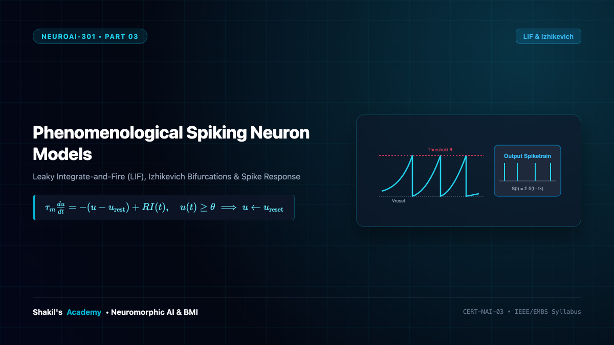
First introduced conceptually by Louis Lapicque in 1907, the LIF model treats the sub-threshold neuron as a simple parallel resistor-capacitor (RC) circuit. The membrane potential (u(t)) evolves according to the linear first-order differential equation:
[
au_m rac{du}{dt} = -(u(t) – u_{ ext{rest}}) + R , I(t)
]
where ( au_m = R C_m) is the membrane time constant (typically (10 ext{ to } 30 ext{ ms})), (u_{ ext{rest}}) is the resting membrane potential (typically (-70 ext{ mV})), and (R) is the input resistance.
Instead of modeling the biophysical ion channel currents during a spike, the model employs a discontinuous, algorithmic reset rule:
[
ext{If } u(t) ge artheta, quad ext{then } begin{cases} ext{Fire Spike at } t = t^{(k)} u(t^+) = u_{ ext{reset}} nd{cases}
]
Following a spike, the potential is clamped at (u_{ ext{reset}}) for an absolute refractory period (Delta_{ ext{abs}}) (typically (1 ext{ to } 3 ext{ ms})), during which the ODE is paused.
2. Analytic Solution and Firing Frequency
For a constant input current (I(t) = I_0) satisfying the threshold condition (u_{ ext{rest}} + R I_0 > artheta), integrating the LIF equation yields the membrane trajectory:
[
u(t) = u_{ ext{rest}} + R I_0 + left( u_{ ext{reset}} – (u_{ ext{rest}} + R I_0)
ight) e^{-t / au_m}
]
The inter-spike interval (T) is found by setting (u(T) = artheta):
[
T = Delta_{ ext{abs}} + au_m ln left( rac{R I_0 + u_{ ext{rest}} – u_{ ext{reset}}}{R I_0 + u_{ ext{rest}} – artheta}
ight)
]
Inverting (T) gives the firing frequency curve (f(I) = 1/T), reproducing the characteristic gain function of biological cortical pyramidal cells.
3. The Izhikevich Model: Rich Dynamics in Two Variables
In 2003, Eugene Izhikevich formulated an astonishingly elegant 2D non-linear model that reproduces virtually all 20 known neuro-computational firing patterns (regular spiking, intrinsically bursting, chattering, fast spiking, thalamo-cortical oscillations) using only a few basic operations per timestep:
[
rac{dv}{dt} = 0.04 v^2 + 5v + 140 – u + I
]
[
rac{du}{dt} = a(bv – u)
]
with the auxiliary reset condition:
[
ext{if } v ge +30 ext{ mV}, quad ext{then } begin{cases} v leftarrow c u leftarrow u + d nd{cases}
]
| Neuron Firing Class | Parameter (a) (Decay) | Parameter (b) (Sensitivity) | Parameter (c) (v-reset) | Parameter (d) (u-bump) |
|---|---|---|---|---|
| Regular Spiking (RS) | 0.02 | 0.2 | -65 mV | 8 |
| Intrinsically Bursting (IB) | 0.02 | 0.2 | -55 mV | 4 |
| Chattering (CH) | 0.02 | 0.2 | -50 mV | 2 |
| Fast Spiking (FS) | 0.1 | 0.2 | -65 mV | 2 |
4. The Spike Response Model (SRM)
Gerstner generalized the LIF model into an integral representation known as the Spike Response Model (SRM). The membrane potential is expressed directly as a sum of kernel convolutions over past spike history:
[
u(t) = ta(t – hat{t}) + int_0^infty kappa(s) I(t – s) ds + sum_{i, k} w_i psilon(t – t_i^{(k)})
]
where (ta(s)) is the post-spike hyperpolarization kernel, (kappa(s)) is the input filter, and (psilon(s)) is the post-synaptic potential (PSP) response kernel. This formulation eliminates continuous ODE integration, enabling fast analytical event-driven simulations in digital hardware.