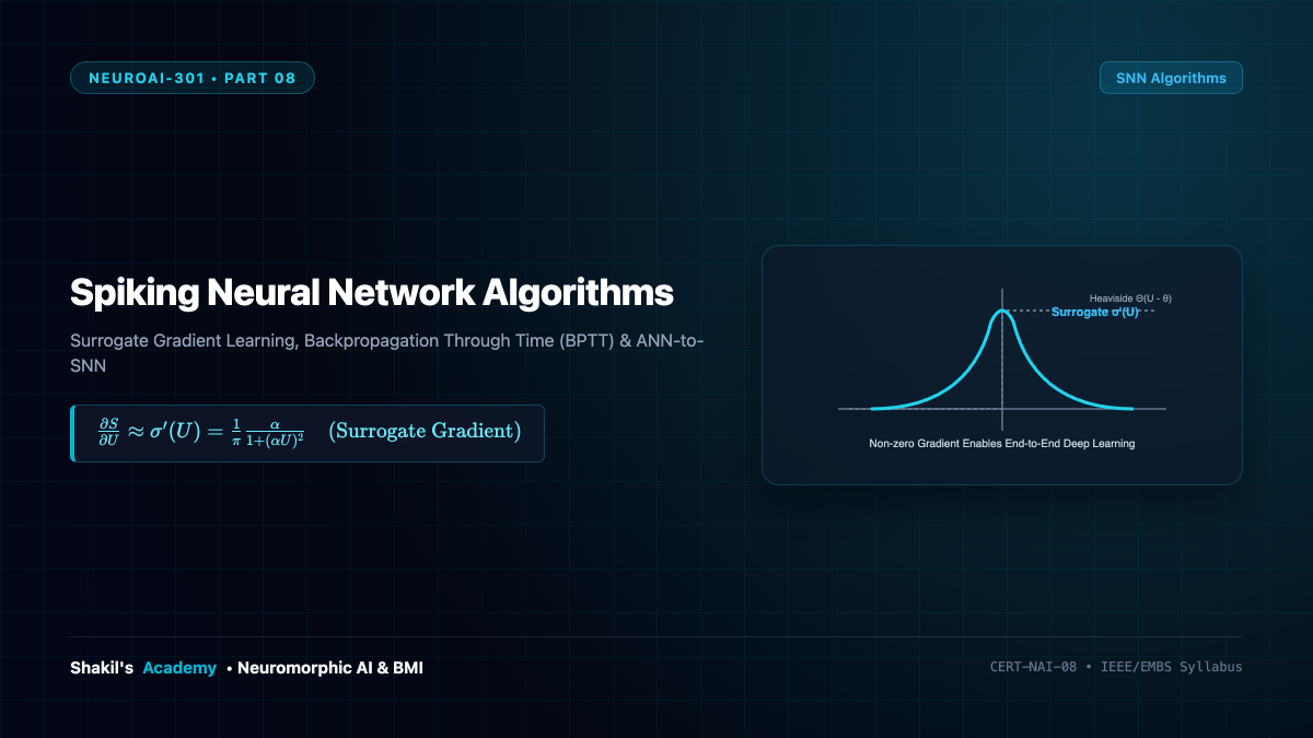
Artificial Neural Networks (ANNs) have revolutionized machine learning by optimizing continuous, differentiable activation functions (ReLU, GELU, Softmax) using stochastic gradient descent and Backpropagation. In Spiking Neural Networks (SNNs), however, neurons communicate using all-or-none binary spikes governed by the Heaviside step function: (Theta(u – artheta)). The derivative of this step function is zero everywhere except at the threshold, where it explodes into a Dirac delta function: (Theta'(x) = delta(x)). This Non-Differentiability Bottleneck long prevented deep backpropagation in SNNs, until the revolutionary development of Surrogate Gradient Learning and rigorous ANN-to-SNN conversion.
1. The Non-Differentiable Spike Generation Dilemma
In a discretized Leaky Integrate-and-Fire (LIF) network with membrane time constant ( au_m) and decay factor (beta = xp(-Delta t / au_m)), the membrane potential (u_i[t]) and output spike (s_i[t] in {0, 1}) update at timestep (t) as:
[
u_i[t] = beta u_i[t-1] (1 – s_i[t-1]) + sum_j w_{ij} s_j[t] + b_i
]
[
s_i[t] = Theta(u_i[t] – artheta)
]
Applying the chain rule to compute the gradient of a loss function (mathcal{L}) with respect to synaptic weight (w_{ij}) via Backpropagation Through Time (BPTT):
[
rac{partial mathcal{L}}{partial w_{ij}} = sum_{t} rac{partial mathcal{L}}{partial s_i[t]} cdot rac{partial s_i[t]}{partial u_i[t]} cdot rac{partial u_i[t]}{partial w_{ij}}
]
The middle term is the derivative of the Heaviside step function:
[
rac{partial s_i[t]}{partial u_i[t]} = rac{dTheta(u_i[t] – artheta)}{du} = begin{cases} 0 & ext{if } u_i[t]
e artheta infty & ext{if } u_i[t] = artheta nd{cases}
]
In standard backpropagation, the gradient is zero almost everywhere, completely halting learning (the dead neuron problem).
2. Surrogate Gradient Learning: The Continuous Relaxation Breakthrough
Pioneered by Neftci, Zenke, and Bellec (2018–2019), Surrogate Gradient Learning resolves this paradox through an ingenious split computation:
- Forward Pass: The exact non-linear, discontinuous biological thresholding is retained: (s_i[t] = Theta(u_i[t] – artheta)). This ensures the network preserves true binary event-driven sparsity.
- Backward Pass: The non-differentiable Dirac delta is replaced by the smooth derivative of a continuous surrogate function:
[
rac{partial s_i[t]}{partial u_i[t]} approx sigma'(u_i[t] – artheta)
]
| Surrogate Function Name | Surrogate Expression (sigma(x)) | Surrogate Derivative (sigma'(x)) Used in Backward Pass |
|---|---|---|
| Fast Sigmoid | (rac{x}{1 + alpha |x|}) | (sigma'(x) = rac{1}{(1 + alpha |x|)^2}) |
| Arctangent | (rac{1}{pi} arctan(alpha x) + rac{1}{2}) | (sigma'(x) = rac{1}{pi} rac{alpha}{1 + (alpha x)^2}) |
| Rectangular (Piecewise Linear) | Piecewise linear ramp | (sigma'(x) = rac{1}{alpha} cdot mathbb{I}(|x| < rac{alpha}{2})) |
| Gaussian Derivative | Error function ( ext{erf}(x)) | (sigma'(x) = rac{1}{sqrt{2pi}alpha} xpleft(-rac{x^2}{2alpha^2} ight)) |
Surrogate gradients allow modern deep learning frameworks (PyTorch, snnTorch, SpikingJelly) to backpropagate directly across thousands of time steps, achieving accuracy parity with ResNets and Vision Transformers while requiring (10 imes) to (50 imes) less computational energy.
3. ANN-to-SNN Conversion Mechanics
An alternative paradigm avoids temporal training entirely by pre-training a standard continuous ReLU ANN, and then mapping its weights directly to an equivalent SNN:
- In a ReLU network, the activation is (a = max(0, W x + b)).
- In an integrate-and-fire SNN, over an observation window of (T) timesteps, the average firing rate is:
[
r = rac{N_{ ext{spikes}}}{T} = rac{1}{T artheta} sum_{t=1}^T I[t] approx rac{W x}{artheta}
] - By scaling the thresholds (artheta) layer-by-layer (Data-Based Threshold Normalization) to match the maximum activation observed across calibration sets ((artheta_l = max_{x} a_l(x))), the SNN reproduces the continuous activations with near-zero accuracy degradation.
While ANN-to-SNN conversion enables rapid deployment of pre-trained models to neuromorphic chips, direct surrogate gradient training is superior for exploiting temporal dynamics and minimizing latency ((T le 4) timesteps vs (T ge 64) for converted networks).