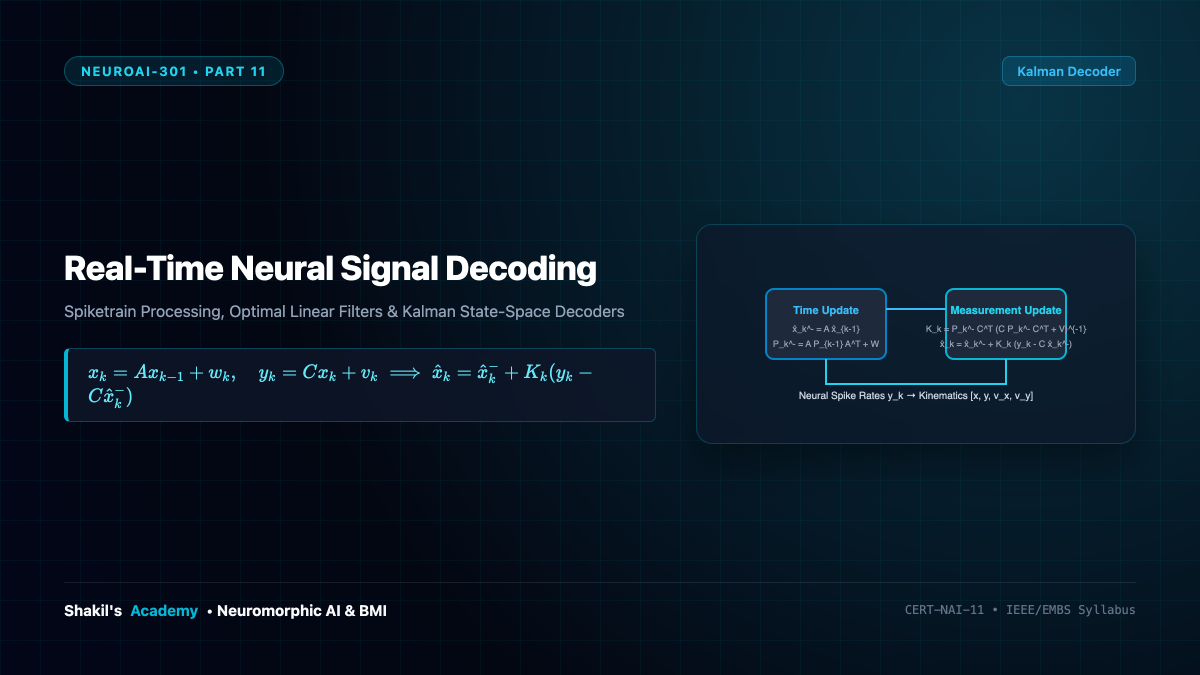
Raw electrophysiological recordings consist of noisy continuous voltage traces corrupted by electrical line hum, muscle artifact (EMG), and movement transients. The core mission of a Brain-Machine Interface (BMI) decoding engine is to extract meaningful low-dimensional kinematic or symbolic control signals from these high-dimensional neural representations in real time ((< 20 ext{ ms}) loop latency). This part details the complete algorithmic decoding pipeline: from spike detection and thresholding to Wiener Optimal Filters and recursive Kalman State-Space Decoders.
1. The Front-End Neural Processing Pipeline
Before statistical decoding algorithms can estimate intention, raw extracellular voltages (v(t)) undergo three consecutive preprocessing steps:
- Digital Bandpass Filtering: A 4th-order Butterworth bandpass filter ((300 ext{ Hz} ext{ to } 6 ext{ kHz})) isolates action potential spikes from low-frequency Local Field Potentials (LFPs).
- Spike Detection via Adaptive Energy Thresholding: Spikes are detected whenever the filtered signal crosses an amplitude threshold (artheta) calibrated to the robust background noise estimation (Quiroga et al.):
[
artheta = 4 imes sigma_n, qquad sigma_n = ext{median}left( rac{|v(t)|}{0.6745}
ight)
] - Spike Binning and Rate Estimation: Spikes are counted in sliding non-overlapping temporal bins (typically (Delta t = 20 ext{ to } 50 ext{ ms})), yielding instantaneous firing rate vector (mathbf{y}_k in mathbb{R}^M) across (M) neural channels at timestep (k).
2. Optimal Linear Filters: The Wiener Filter
The simplest effective kinematics decoder is the multi-lag Wiener Linear Filter, which models intended kinematic velocity (mathbf{x}_k = [v_x, v_y]^T) as a linear combination of firing rates across the past (N_{ ext{lags}}) time intervals:
[
hat{mathbf{x}}_k = sum_{ au=0}^{N_{ ext{lags}}-1} mathbf{W}_ au mathbf{y}_{k – au} + mathbf{b} = mathbf{W}_{ ext{ext}} mathbf{Y}_k
]
Minimizing the mean squared error (MSE) (mathbb{E}[|mathbf{x}_k – hat{mathbf{x}}_k|^2]) over training data yields the analytical Wiener-Hopf solution:
[
mathbf{W}_{ ext{ext}} = left( mathbf{Y} mathbf{Y}^T + lambda mathbf{I}
ight)^{-1} mathbf{Y} mathbf{X}^T
]
where (lambda mathbf{I}) is an (L_2) Tikhonov regularization term preventing overfitting. While computationally trivial, Wiener filters are purely feedforward and do not enforce physical momentum or kinematic smoothness constraints.
3. The Kalman State-Space Filter Decoder
Pioneered for BMIs by Wu, Gao, Bienenstock, Donoghue, and Black (2002–2006), the Kalman Filter provides a mathematically principled Bayesian framework that unifies a model of physical limb movement with a generative model of neural firing.
Step A: State Kinematics Model (Prior)
The kinematic state vector (mathbf{x}_k = [p_x, p_y, v_x, v_y, 1]^T) evolves according to linear Newtonian dynamics driven by Gaussian process noise (mathbf{w}_k sim mathcal{N}(0, mathbf{W})):
[
mathbf{x}_k = mathbf{A} mathbf{x}_{k-1} + mathbf{w}_k
]
where (mathbf{A}) captures inertia and velocity damping.
Step B: Neural Observation Model (Likelihood)
The neural firing rate vector (mathbf{y}_k in mathbb{R}^M) is linearly related to the kinematic state, corrupted by Gaussian observation noise (mathbf{v}_k sim mathcal{N}(0, mathbf{V})):
[
mathbf{y}_k = mathbf{C} mathbf{x}_k + mathbf{v}_k
]
where (mathbf{C} in mathbb{R}^{M imes 5}) represents the cosine tuning curves (Georgopoulos directional preference) of the motor cortical population.
Step C: The Recursive Kalman Loop
At every 20 ms timestep, the decoder executes two recursive steps:
[
hat{mathbf{x}}_k^- = mathbf{A} hat{mathbf{x}}_{k-1}, qquad mathbf{P}_k^- = mathbf{A} mathbf{P}_{k-1} mathbf{A}^T + mathbf{W}
]
2. Measurement Update (Correct):
[
mathbf{K}_k = mathbf{P}_k^- mathbf{C}^T left( mathbf{C} mathbf{P}_k^- mathbf{C}^T + mathbf{V}
ight)^{-1}
]
[
hat{mathbf{x}}_k = hat{mathbf{x}}_k^- + mathbf{K}_k left( mathbf{y}_k – mathbf{C} hat{mathbf{x}}_k^-
ight)
]
[
mathbf{P}_k = left( mathbf{I} – mathbf{K}_k mathbf{C}
ight) mathbf{P}_k^-
]
The Kalman Gain (mathbf{K}_k) optimally balances trust between physical kinematic continuity ((mathbf{P}_k^-)) and noisy neural observation ((mathbf{V})), producing exceptionally smooth, jitter-free cursor and robotic arm trajectories.
4. Non-Linear Generalizations: Unscented Kalman and Point-Process Filters
To overcome linear assumptions, modern clinical decoders utilize advanced extensions:
- Unscented Kalman Filter (UKF): Propagates deterministically selected sigma points through non-linear kinematic transforms (e.g., robotic arm joint angle forward kinematics).
- Point-Process Generalized Linear Models (PP-GLM): Replaces the Gaussian firing rate assumption with the exact Poisson likelihood of individual spike timestamps, updating state estimates continuously spike-by-spike without needing artificial temporal bins.