Open-loop dynamics feedforward fails in the physical world due to unmodeled friction, payload mass uncertainty, and external disturbances. High-performance trajectory execution requires closed-loop feedback motion control. By exploiting the analytical structure of manipulator dynamics, Computed Torque Control linearizes non-linear robot equations into decoupled linear systems. Furthermore, when interacting with physical environments or humans, pure position control is hazardous; robots must transition to Impedance Control, modulating dynamic mechanical compliance.
1. Computed Torque Control (Feedback Linearization)
Recall the non-linear manipulator dynamics: (M(q)ddot{q} + C(q,dot{q})dot{q} + g(q) = au). Because the mass matrix (M(q)) is invertible everywhere, we can design a non-linear state feedback control law:
[
au = M(q) u + C(q,dot{q})dot{q} + g(q)
]
Where (u in mathbb{R}^n) is a synthetic auxiliary control input. Substituting this control law into the equations of motion completely cancels the non-linear Coriolis, centrifugal, and gravitational forces, reducing the entire coupled multi-body robot to a trivial set of (n) decoupled unit double integrators:
[
ddot{q} = u
]
Choosing (u) as a proportional-derivative (PD) tracking feedback with feedforward desired acceleration (ddot{q}_d):
[
u = ddot{q}_d + K_v (dot{q}_d – dot{q}) + K_p (q_d – q)
]
The closed-loop tracking error (e(t) = q_d(t) – q(t)) satisfies the linear second-order error dynamics:
[
ddot{e} + K_v dot{e} + K_p e = 0
]
Selecting positive-definite diagonal gain matrices (K_p = ext{diag}(omega_n^2)) and (K_v = ext{diag}(2zetaomega_n)) guarantees exponential asymptotic convergence of tracking error to zero ((e(t) o 0)) with desired natural frequency (omega_n) and damping ratio (zeta).
2. Khatib’s Operational Space Formulation
Controlling a robot in joint space requires pre-computing inverse kinematics. In 1987, Oussama Khatib revolutionized robot manipulation by formulating the dynamics directly in Operational (Task) Space (x = f(q)):
[
Lambda(x) ddot{x} + mu(x, dot{x}) + p(x) = F
]
Where:
- (Lambda(x) = (J M^{-1} J^T)^{-1}): The operational space inertia matrix.
- (mu(x, dot{x})): Operational space Coriolis and centrifugal force vector.
- (p(x) = Lambda J M^{-1} g): Operational space gravity force.
- (F in mathbb{R}^6): Control wrench commanded directly at the end-effector.
Joint torques are generated dynamically via ( au = J^T(q) F + [I – J^T bar{J}^T] au_{ ext{null}}), where (bar{J} = M^{-1} J^T Lambda) is the dynamically consistent generalized inverse.
3. Neville Hogan’s Impedance Control
When an industrial arm operating under stiff position control encounters an unexpected obstacle or human hand, tracking error spikes, prompting the feedback controller to output maximum torque, crushing the obstacle. To achieve safe contact, Neville Hogan (1985) introduced Impedance Control.
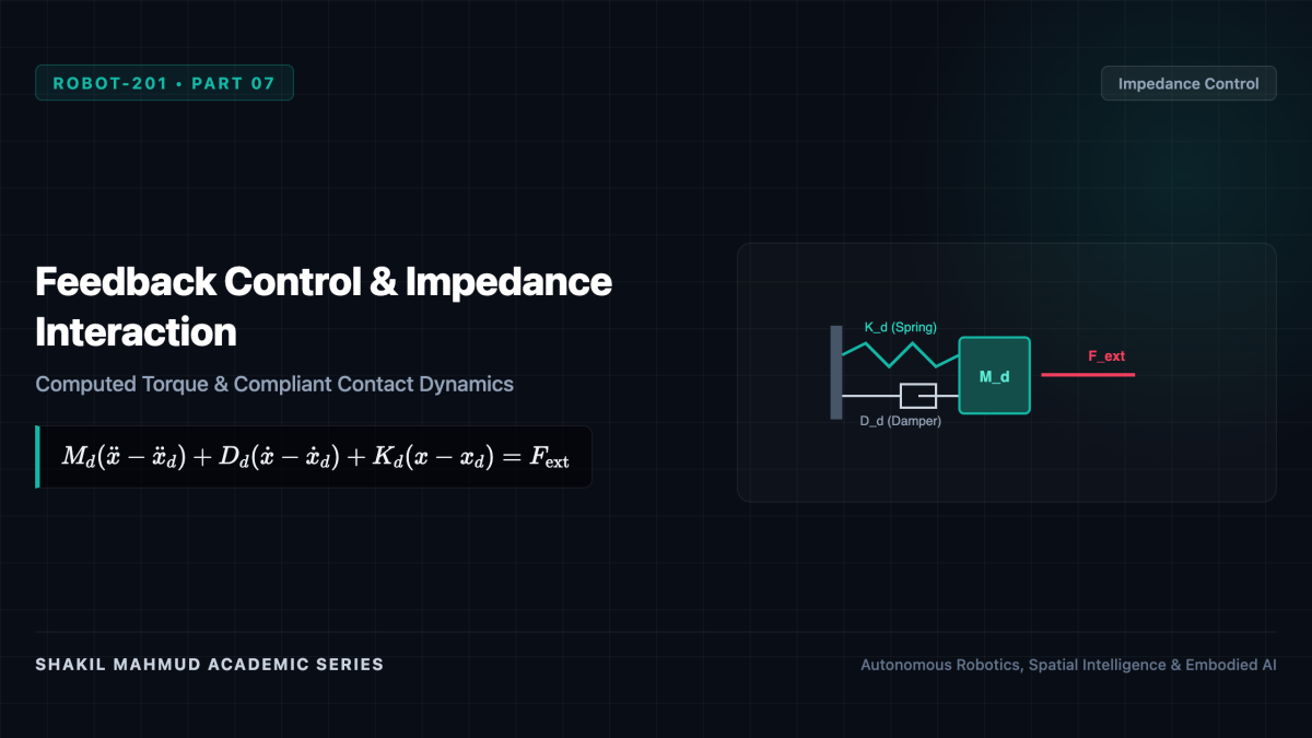
Instead of regulating position or force independently, impedance control regulates the dynamic relationship between external contact force (F_{ ext{ext}}) and motion error (e = x – x_d):
[
M_d ddot{e} + D_d dot{e} + K_d e = F_{ ext{ext}}
]
Where:
- (M_d): Desired virtual mass matrix.
- (D_d): Desired virtual damping matrix.
- (K_d): Desired virtual stiffness matrix.
The robot behaves exactly like a programmable mechanical spring-damper. If external force pushes against the gripper, the robot compliantly gives way according to stiffness (K_d). Once the contact ceases, the robot smoothly returns to its target trajectory, enabling seamless assembly, polishing, wiping, and safe physical human-robot collaboration (cobots).