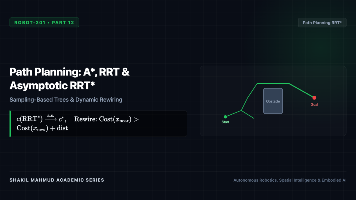
Given a metric map and an accurate state estimate, how does a robot compute a collision-free motion trajectory from its starting configuration (q_{ ext{start}}) to a goal region (q_{ ext{goal}})? This is the problem of motion planning. Operating within the robot’s high-dimensional Configuration Space ((mathcal{C})-Space), planning algorithms navigate the continuum between discrete graph search (Dijkstra, (A^*)) and continuous randomized sampling (RRT, ( ext{RRT}^*)).
1. The Geometry of Configuration Space (C-Space)
A physical robot occupies finite volume in workspace (mathcal{W} = mathbb{R}^3). Checking collisions between complex 3D meshes is computationally prohibitive. In 1979, Tomás Lozano-Pérez introduced the Configuration Space ((mathcal{C})-space): mapping the robot’s geometric morphology into an abstract (d)-dimensional space of generalized coordinates (q in mathcal{C}), where the robot shrinks to an infinitesimal point (mathbf{0}).
Physical workspace obstacles (mathcal{O}_i) are dilated by the robot’s geometry via the Minkowski sum to form (mathcal{C})-space obstacles:
[
mathcal{C}_{ ext{obs}} = bigcup_i left{ q in mathcal{C} middle| mathcal{A}(q) cap mathcal{O}_i
eq mptyset
ight}, quad mathcal{C}_{ ext{free}} = mathcal{C} setminus mathcal{C}_{ ext{obs}}
]
Motion planning is thereby reduced to the clean topological problem of finding a continuous path (gamma: [0, 1] o mathcal{C}_{ ext{free}}) such that (gamma(0) = q_{ ext{start}}) and (gamma(1) = q_{ ext{goal}}).
2. Discrete Graph Search: Dijkstra vs. A*
Discretizing (mathcal{C}_{ ext{free}}) into a grid or visibility graph allows shortest-path graph search:
- Dijkstra’s Algorithm: Expands outward uniformly in all directions, evaluating total cost-to-come (g(n)). Dijkstra guarantees the globally optimal shortest path but explores wasteful regions far from the goal.
- (A^*) Search: Directs the search toward the goal using an evaluation priority function (f(n) = g(n) + h(n)), where (h(n)) is an estimated cost-to-go heuristic.
If the heuristic (h(n)) is admissible ((h(n) le h^*(n)), never overestimating true remaining cost) and consistent ((h(n) le c(n, n’) + h(n’))), (A^*) is provably optimal and expands the minimum possible number of nodes.
3. High-Dimensional Sampling: RRT vs. RRT*
For high-dimensional manipulators ((n ge 6) joints), grid discretization suffers from Bellman’s curse of dimensionality ((mathcal{O}(k^n)) cells). In 1998, Steven LaValle introduced Rapidly-exploring Random Trees (RRT):
- Sample a random configuration (q_{ ext{rand}} in mathcal{C}_{ ext{free}}).
- Find the nearest tree vertex (q_{ ext{near}} = argmin_{v in V} |v – q_{ ext{rand}}|).
- Steer a step (Delta q) toward (q_{ ext{rand}}) to create candidate vertex (q_{ ext{new}}). If the segment is collision-free, add (q_{ ext{new}}) to tree (mathcal{T}).
RRT exhibits a natural Voronoi bias, rapidly exploring open spaces, and is probabilistically complete (probability of finding a solution approaches 1 as samples (N o infty)). However, RRT paths are jagged, jerky, and severely sub-optimal.
4. Sertac Karaman and Emilio Frazzoli’s RRT*
In 2011, Karaman and Frazzoli proved that standard RRT converges to a sub-optimal path with probability 1. They introduced ( ext{RRT}^*), introducing two critical algorithmic operations inside a neighborhood ball of radius (r_N propto (log N / N)^{1/d}):
- Best Parent Selection: Instead of connecting (q_{ ext{new}}) strictly to (q_{ ext{near}}), ( ext{RRT}^*) examines all nearby neighbors (X_{ ext{near}}) and chooses the parent that minimizes total cost from root:
[
q_{min} = argmin_{q in X_{ ext{near}}} left( ext{Cost}(q) + |q – q_{ ext{new}}|
ight)
] - Local Rewiring: For every neighbor (q in X_{ ext{near}}), ( ext{RRT}^*) checks if routing through (q_{ ext{new}}) offers a lower cost than its existing parent:
[
ext{If } ext{Cost}(q_{ ext{new}}) + |q_{ ext{new}} – q| < ext{Cost}(q), quad ext{rewire parent of } q ext{ to } q_{ ext{new}}
]
Through recursive rewiring, ( ext{RRT}^*) achieves asymptotic optimality: as the number of samples approaches infinity, the cost of the generated trajectory converges almost surely to the globally optimal shortest path ((c( ext{RRT}^*) xrightarrow{ ext{a.s.}} c^*)).