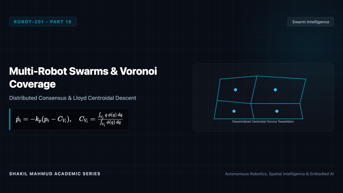
While a single sophisticated robot is fragile, expensive, and limited by local sensor range, nature demonstrates that hundreds of simple, decentralized agents—such as ant colonies, bird flocks, and schools of fish—can accomplish astonishing collective intelligence. Multi-Robot Swarms operate without central points of failure, relying on local peer-to-peer communication graphs to achieve distributed consensus, spatial environmental coverage via Centroidal Voronoi Tessellations, and dynamic collision-free flocking.
1. Algebraic Graph Theory and Communication Topologies
A swarm of (N) robots is represented by an undirected communication graph (mathcal{G} = (mathcal{V}, mathcal{E})), where edges ((i, j) in mathcal{E}) represent active peer-to-peer wireless links. The topology is formalized by the Graph Laplacian Matrix (L in mathbb{R}^{N imes N}):
[
L = D – A
]
Where (A) is the adjacency matrix ((A_{ij} = 1) if connected, (0) otherwise) and (D = ext{diag}( ext{deg}(i))) is the diagonal degree matrix. Fundamental algebraic properties of (L) include:
- The row sums are identically zero: (L mathbf{1} = mathbf{0}).
- The eigenvalues are non-negative: (0 = lambda_1 le lambda_2 le cdots le lambda_N).
- Algebraic Connectivity ((lambda_2)): By Miroslav Fiedler (1973), the second smallest eigenvalue (lambda_2(L) > 0) if and only if the communication graph is connected. The magnitude of (lambda_2) dictates the exponential convergence speed of distributed consensus across the entire swarm.
2. Distributed Consensus Protocols
To agree on a common spatial heading, target destination, or environmental measurement (x_i in mathbb{R}^d) without a central master server, each robot updates its state using only local neighbor differences:
[
dot{x}_i(t) = -k sum_{j in mathcal{N}_i} left( x_i(t) – x_j(t)
ight) iff dot{mathbf{x}}(t) = -k L mathbf{x}(t)
]
Under connected topologies, the swarm exponentially converges to the average consensus:
[
x_i(t) o rac{1}{N} sum_{j=1}^N x_j(0) quad ext{at rate } e^{-k lambda_2 t}
]
3. Optimal Spatial Coverage: Centroidal Voronoi Tessellation (CVT)
In search-and-rescue, environmental monitoring, or agricultural spraying, (N) mobile robots must deploy across a 2D domain (Q) to maximize sensor coverage. Given robot positions (p = [p_1, dots, p_N]), the domain partitions into Voronoi Cells (V_i):
[
V_i = left{ q in Q middle| |q – p_i| le |q – p_j| quad orall j
eq i
ight}
]
Let (phi(q) ge 0) represent an environmental density distribution (e.g., wildfire probability). Jorge Cortés et al. (2004) formulated the locational coverage cost function:
[
mathcal{H}(p_1, dots, p_N) = sum_{i=1}^N int_{V_i} |q – p_i|^2 phi(q) , dq
]
Differentiating with respect to robot position (p_i) yields the gradient:
[
rac{partial mathcal{H}}{partial p_i} = 2 M_{V_i} left( p_i – C_{V_i}
ight)
]
Where (M_{V_i} = int_{V_i} phi(q) dq) is the cell mass and (C_{V_i}) is the geometric center of mass (centroid) of cell (V_i):
[
C_{V_i} = rac{int_{V_i} q , phi(q) , dq}{int_{V_i} phi(q) , dq}
]
By executing Distributed Lloyd’s Algorithm—where each robot simply measures its neighbors’ distances to construct its local cell and drives toward its own centroid (dot{p}_i = -k (p_i – C_{V_i}))—the swarm converges asymptotically to a Centroidal Voronoi Configuration, guaranteeing mathematically optimal sensory coverage with zero central control.
4. Reynolds Flocking Dynamics
For dynamic transit through obstacle fields, swarms execute Craig Reynolds’ distributed flocking rules (Olfati-Saber, 2006):
- Separation: Repulsive potential fields prevent collisions between close neighbors ((r < r_{ ext{safe}})).
- Alignment: Velocity consensus aligns heading and speed with neighbors ((v_i o v_j)).
- Cohesion: Attractive potential pulls distant neighbors together, preserving swarm connectivity.
Swarm intelligence enables hundreds of micro-drones or autonomous underwater vehicles (AUVs) to map subterranean caves, explore disaster zones, and defend maritime coastlines with fault-tolerant resilience.