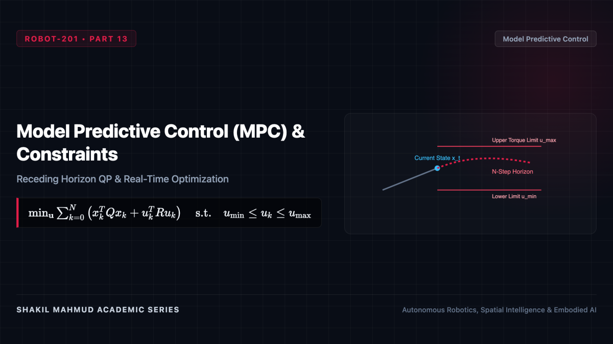
Classical feedback controllers (PID, LQR) are fundamentally myopic: they react purely to current tracking error without foresight and struggle with hard physical inequality constraints (such as actuator torque saturation, joint angle limits, and collision boundaries). Model Predictive Control (MPC) fundamentally transforms motion control into an online, real-time mathematical optimization problem: repeatedly solving a constrained finite-horizon optimal control problem and applying only the first step of the computed control trajectory in a receding horizon fashion.
1. The Discrete-Time Constrained Optimal Control Formulation
Consider a discrete-time dynamical system (x_{k+1} = f(x_k, u_k)) with state (x in mathbb{R}^n) and actuator inputs (u in mathbb{R}^m). At each sampling instant (t), MPC predicts system evolution over a future horizon of (N) steps by solving the following optimization problem:
[
min_{mathbf{u} = {u_0, u_1, dots, u_{N-1}}} left[ x_N^T P x_N + sum_{k=0}^{N-1} left( x_k^T Q x_k + u_k^T R u_k
ight)
ight]
]
Subject to:
[
x_0 = x(t) quad ( ext{Current state feedback})
]
[
x_{k+1} = A x_k + B u_k quad ( ext{System dynamics})
]
[
u_{min} le u_k le u_{max} quad ( ext{Actuator torque/voltage saturation})
]
[
x_{min} le x_k le x_{max} quad ( ext{Safety envelopes and joint limits})
]
[
x_N in mathcal{X}_f quad ( ext{Terminal invariant set})
]
Where (Q ge 0) penalizes state deviation, (R > 0) penalizes control effort, and (P) is the terminal cost matrix derived from the unconstrained discrete algebraic Riccati equation (DARE).
2. Receding Horizon Principle
Although the optimization yields an optimal sequence of (N) control actions (mathbf{u}^* = {u_0^*, u_1^*, dots, u_{N-1}^*}):
- Only the very first control action (u(t) = u_0^*) is physically commanded to the robot’s motor drives.
- The robot advances one time-step (Delta t), reaching a new state (x(t + Delta t)).
- The horizon shifts forward by one step, a new state measurement is acquired, and the entire optimization is resolved from the new initial condition.
This closed-loop feedback mechanism provides exceptional robustness against modeling errors and unpredicted environmental disturbances.
3. Fast Quadratic Programming (QP) Solvers
For linear systems with polyhedral constraints, the MPC formulation is condensed into a convex Quadratic Program (QP):
[
min_z rac{1}{2} z^T H z + g^T z quad ext{subject to } l le C z le u
]
Where (z = [u_0^T, dots, u_{N-1}^T]^T) has dimension (N cdot m). To solve this QP at 500 Hz to 1 kHz on embedded processors, modern robotics relies on first-order operator-splitting algorithms—most notably ADMM (Alternating Direction Method of Multipliers) implemented in open-source solvers like OSQP. ADMM decouples dynamic equality constraints from inequality box bounds, computing millisecond solutions even on microcontrollers.
4. Non-Linear MPC and Differential Dynamic Programming (DDP)
When controlling highly non-linear systems (e.g., acrobatic drones or legged humanoids), linear approximations fail. Non-Linear Model Predictive Control (NMPC) optimizes through non-linear dynamics using second-order trajectory optimization algorithms like Differential Dynamic Programming (DDP) and Iterative LQR (iLQR).
By quadratizing the cost and linearizing dynamics along a nominal trajectory, iLQR computes backward Riccati sweeps with (mathcal{O}(N)) linear complexity, allowing humanoids to dynamically balance, recover from violent pushes, and jump over hurdles in real time.