Cameras are the richest, lightest, and cheapest sensors in robotics: a single CMOS sensor streams millions of colorful spatial rays per second. Visual Odometry (VO) and Visual SLAM (V-SLAM) recover the 6-DoF trajectory of a camera alongside a 3D structural reconstruction of the environment solely from incoming image streams. The field bifurcates into two distinct mathematical philosophies: feature-based methods tracking sparse geometric keypoints, and direct methods optimizing continuous photometric pixel intensities.
1. Feature-Based Visual SLAM: Epipolar Geometry
In classical feature-based visual SLAM (e.g., ORB-SLAM3), distinct salient corners (ORB, SIFT, SuperPoint) are detected and matched across consecutive frames (I_{t-1}) and (I_t). The geometric relationship between two calibrated camera views is governed by the Essential Matrix (E in mathbb{R}^{3 imes 3}):
[
E = [t]_{ imes} R, quad ext{satisfying the epipolar constraint: } x_2^T E x_1 = 0
]
Where (x_1, x_2) are normalized homogeneous camera coordinates. Decomposing (E) via Singular Value Decomposition (SVD) recovers the relative rotation (R in ext{SO}(3)) and translation direction (t in mathbb{S}^2) up to an arbitrary scale factor (in monocular SLAM).
2. Bundle Adjustment (BA) and Reprojection Error
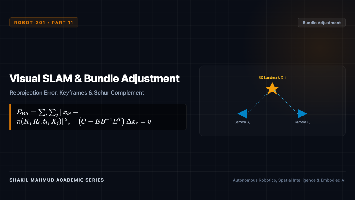
To refine camera poses and 3D landmark positions globally, Visual SLAM executes Bundle Adjustment (BA). BA minimizes the sum of squared reprojection errors—the Euclidean pixel distance between the observed 2D feature location (x_{ij}) and the camera projection of the 3D map point (X_j in mathbb{R}^3):
[
E_{ ext{BA}} = sum_{i in ext{Frames}} sum_{j in ext{Points}}
ho left( left| x_{ij} – pi(K, T_i, X_j)
ight|^2
ight)
]
Where (pi(K, T_i, X_j)) is the pinhole camera projection function with intrinsic matrix (K), and (
ho(cdot)) is a robust Huber/Tukey loss function rejecting outlier matches.
Because each map point is only observed in a subset of camera keyframes, the Hessian matrix possesses a distinct arrowhead sparse block structure:
[
H = begin{bmatrix} B & E E^T & C nd{bmatrix} begin{bmatrix} Delta x_c Delta x_p nd{bmatrix} = begin{bmatrix} v w nd{bmatrix}
]
Applying the Schur Complement inverts the diagonal point matrix (C) in linear time, reducing the system to the reduced camera bundle equation:
[
left( B – E C^{-1} E^T
ight) Delta x_c = v – E C^{-1} w
]
Solving solely for camera poses (Delta x_c) and back-substituting points (Delta x_p) enables real-time Bundle Adjustment over hundreds of keyframes simultaneously.
3. Direct Methods: Photometric Error Optimization
Feature-based systems discard (95%) of image information by isolating sparse high-gradient corners, failing in textureless environments (blank walls, corridors). In contrast, Direct Visual SLAM (e.g., DSO, LSD-SLAM) operates directly on raw pixel intensities, exploiting the Brightness Constancy Assumption.
The photometric error over pixel patches (mathcal{N}_p) is formulated as:
[
E_{ ext{photo}} = sum_{p in Omega} sum_{q in mathcal{N}_p} w_q left| left( I_j[p’] – b_j
ight) – rac{t_j e^{a_j}}{t_i e^{a_i}} left( I_i[p] – b_i
ight)
ight|_gamma
]
Where (p’) is the projected coordinate of pixel (p) with inverse depth (d_p) into target frame (I_j), and (a, b) are affine brightness parameters modeling exposure and auto-gain variations. Direct methods construct semi-dense or dense 3D surface maps without feature matching, thriving in low-texture industrial environments.