No robot can perceive its true physical state directly. Sensor measurements are corrupted by stochastic noise, actuator commands suffer from wheel slippage and backlash, and unobserved environmental disturbances constantly inject entropy into the system. Autonomous spatial intelligence addresses this fundamental challenge through Probabilistic State Estimation: maintaining a dynamic probability belief distribution (bel(x_t) = p(x_t mid z_{1:t}, u_{1:t})) over all possible robot states conditioned on past control inputs and sensory observations.
1. The Fundamental Recursive Bayesian Filter
State estimation operates via a continuous two-step Markovian recursion grounded in Bayes’ rule:
- Prediction (Time Update): Projects the belief forward using the stochastic motion model (p(x_t mid u_t, x_{t-1})) via the Chapman-Kolmogorov integral:
[
bar{bel}(x_t) = int p(x_t mid u_t, x_{t-1}) , bel(x_{t-1}) , dx_{t-1}
] - Correction (Measurement Update): Modulates the predicted belief by the likelihood of the incoming sensor measurement (z_t) under observation model (p(z_t mid x_t)):
[
bel(x_t) = ta , p(z_t mid x_t) , bar{bel}(x_t)
]
Where (ta = left( int p(z_t mid x_t) bar{bel}(x_t) dx_t
ight)^{-1}) is the normalizing constant.
2. The Extended Kalman Filter (EKF)
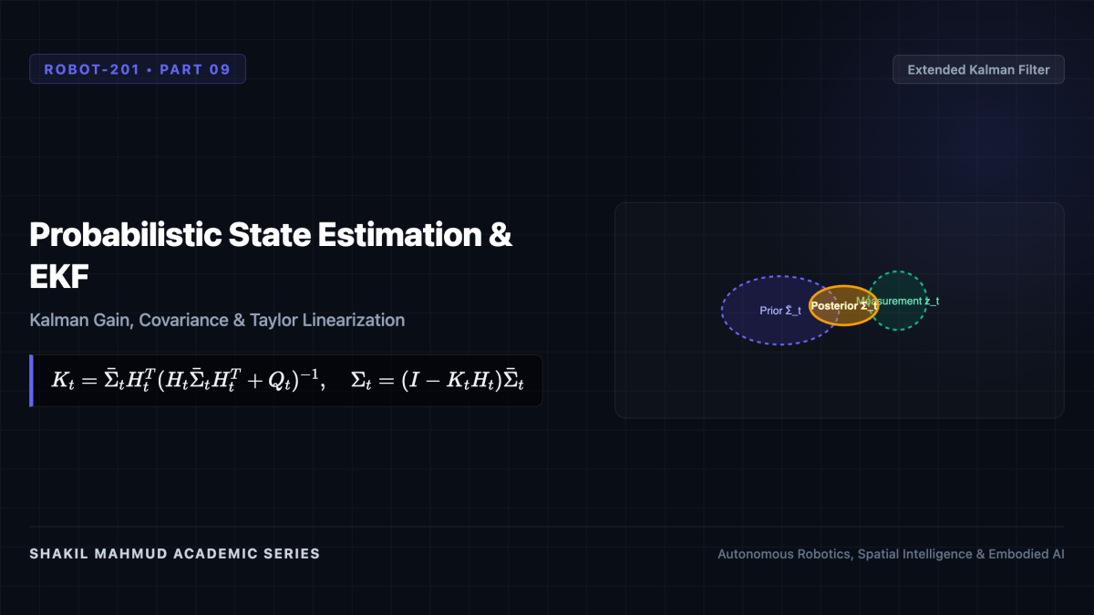
When the state distribution is unimodal and approximately Gaussian ((bel(x_t) sim mathcal{N}(mu_t, Sigma_t))), the Extended Kalman Filter (EKF) handles non-linear dynamics (x_t = f(x_{t-1}, u_t) + w_t) and measurement physics (z_t = h(x_t) + v_t) by evaluating first-order Taylor expansion Jacobians:
[
F_t = left. rac{partial f}{partial x}
ight|_{mu_{t-1}, u_t}, quad H_t = left. rac{partial h}{partial x}
ight|_{bar{mu}_t}
]
The EKF execution equations proceed as follows:
- Prediction:
[
bar{mu}_t = f(mu_{t-1}, u_t), quad bar{Sigma}_t = F_t Sigma_{t-1} F_t^T + Q_t
] - Innovation (Measurement Residual):
[
y_t = z_t – h(bar{mu}_t), quad S_t = H_t bar{Sigma}_t H_t^T + R_t
] - Kalman Gain & Posterior Update:
[
K_t = bar{Sigma}_t H_t^T S_t^{-1}, quad mu_t = bar{mu}_t + K_t y_t, quad Sigma_t = (I – K_t H_t) bar{Sigma}_t
]
The Kalman Gain (K_t) balances prior uncertainty against sensor noise: when sensor covariance (R_t o 0), (K_t o H^{-1}), trusting the sensor completely; when sensor noise explodes ((R_t o infty)), (K_t o 0), trusting purely the motion model.
3. Non-Gaussian Beliefs: Particle Filtering (MCL)
When a robot experiences extreme non-linearities, multimodal hypotheses (e.g., identical corridors), or the kidnapped robot problem, Gaussian assumptions collapse. Monte Carlo Localization (MCL) represents the posterior belief non-parametrically using a set of (M) weighted random samples (particles):
[
mathcal{X}_t = left{ langle x_t^{[m]}, w_t^{[m]}
angle
ight}_{m=1}^M
]
- Sample Motion Model: Draw new state particles by propagating through kinematic odometry with injected noise: (x_t^{[m]} sim p(x_t mid u_t, x_{t-1}^{[m]})).
- Importance Weighting: Assign weights based on LiDAR/sonar raycast likelihood matching against the metric map: (w_t^{[m]} propto p(z_t mid x_t^{[m]})).
- Low-Variance Resampling: Particles with negligible weights die out, while particles with high weights are replicated, concentrating computational effort in regions of high probability density.
MCL enables global localization from scratch without prior position knowledge, robustly recovering from arbitrary kidnapped states in real time.