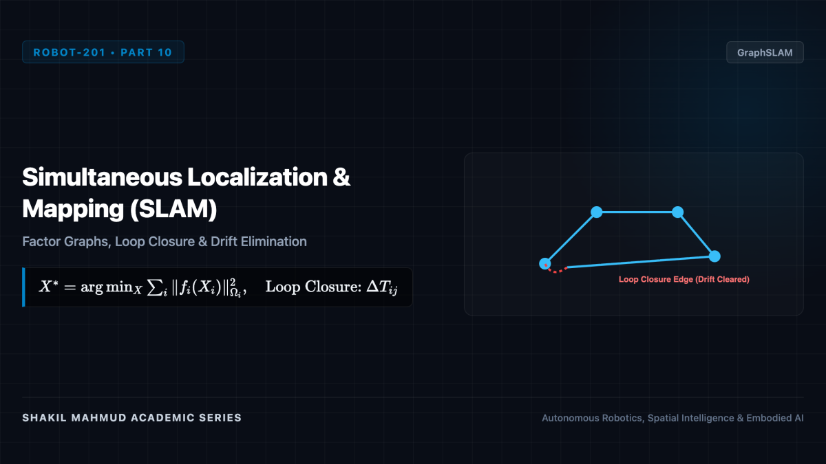
To navigate an unknown environment, a mobile robot must answer two questions simultaneously: “Where am I?” (Localization) and “What does the world look like?” (Mapping). This circular dependency is the famous SLAM (Simultaneous Localization and Mapping) problem: mapping requires accurate localization, while localization requires an accurate map. Modern spatial intelligence addresses SLAM as a massive non-linear graph optimization problem, resolving dead-reckoning drift through Factor Graphs and Loop Closure.
1. The GraphSLAM Paradigm
While early SLAM relied on filtering (filtering out past trajectory poses), modern state-of-the-art systems utilize Graph-based SLAM (GraphSLAM). The robot’s historical trajectory is represented as a graph (mathcal{G} = (mathcal{V}, mathcal{E})):
- Nodes ((x_i in ext{SE}(3))): The discrete spatial poses of the robot at key timestamps (t_1, t_2, dots, t_N), plus 3D coordinates of persistent environmental landmarks (l_j in mathbb{R}^3).
- Edges (Factors): Non-linear probabilistic constraints between nodes derived from odometry, IMU preintegration, or spatial sensor observations.
The optimal trajectory and map correspond to the maximum a posteriori (MAP) state estimate minimizing the sum of Mahalanobis squared residual errors:
[
X^* = argmin_X sum_{k} |r_k(X_k)|^2_{Omega_k} = argmin_X sum_{k} r_k(X_k)^T Omega_k r_k(X_k)
]
Where (Omega_k = Sigma_k^{-1}) is the measurement information matrix.
2. Factor Graphs and Incremental Smoothing (iSAM2)
Formulating SLAM with Factor Graphs makes statistical conditional independencies explicit. As a robot moves, newly added factor edges only connect to recent poses, creating an extraordinarily sparse measurement Jacobian matrix (A).
Solving the linearized normal equations (A^T A Delta X = A^T b) via sparse Cholesky ((L L^T)) or QR factorization allows real-time execution. In Michael Kaess and Frank Dellaert’s landmark iSAM2 (Incremental Smoothing and Mapping) algorithm, the factor graph is converted into a Bayes Tree data structure. When new sensors arrive, only the affected sub-branches of the tree are recalculated, maintaining 100 Hz optimization efficiency over hours of continuous exploration.
3. Loop Closure: Eliminating Accumulated Drift
During exploration, small dead-reckoning errors in wheel odometry and IMU integration compound unbounded over time. The estimated trajectory stretches, bends, and twists away from reality.
The salvation of SLAM is Loop Closure: recognizing when the robot re-enters a previously visited spatial region.
- Place Recognition: Bags-of-Visual-Words (DBoW2), NetVLAD embeddings, or LiDAR Scan Context descriptors match current sensor observations against historical keyframes in real time.
- Geometric Verification: If a topological match is verified via RANSAC point alignment or ICP (Iterative Closest Point), a rigid transformation constraint (Delta T_{ij} in ext{SE}(3)) is created between the current pose (x_i) and the past pose (x_j).
- Global Relaxation: Inserting this non-local loop-closing edge introduces a strong constraint across the graph. Non-linear least squares optimization (e.g., Levenberg-Marquardt in GTSAM or g2o) “relaxes” the entire trajectory, snapping thousands of drifted meters back into rigid global metric alignment.
GraphSLAM with robust loop closure forms the core spatial intelligence inside autonomous delivery rovers, self-driving automobiles, and automated warehouse AGVs.