Plate tectonics is the unifying grand theory of the Earth sciences. It integrates continental drift, seafloor spreading, paleomagnetism, and deep-mantle geodynamics into a single mathematically self-consistent kinematic framework. Across geological time, rigid lithospheric plates drift across the globe, opening ocean basins and collating supercontinents in a continuous 500-million-year tempo known as the Wilson Cycle.
1. Spherical Plate Kinematics and Euler Rotation Vectors
By Euler’s fixed-point theorem, any displacement of a rigid spherical shell on the surface of a sphere is mathematically equivalent to a pure rotation about a fixed diameter through the planetary center. The relative linear velocity (mathbf{v}) of plate (A) relative to plate (B) at any surface position (mathbf{r}) is given by the cross product:
[
mathbf{v}_{A/B}(mathbf{r}) = boldsymbol{omega}_{A/B} imes mathbf{r}
]
where (boldsymbol{omega}_{A/B} = (lambda_E, phi_E, Omega)) is the Euler pole of rotation, characterized by latitude (lambda_E), longitude (phi_E), and angular velocity (Omega) (in ( ext{deg/Myr}) or ( ext{rad/s})). The magnitude of relative motion varies as the sine of angular distance (Delta) from the Euler pole:
[
v = Omega , R_oplus sinDelta
]
Consequently, plate velocity is zero at the Euler pole and reaches a maximum along the rotation equator ((Delta = 90^circ)). Transform faults trace small circles of concentric latitude centered on the Euler pole, providing an unambiguous geometric test for determining relative plate trajectories.
2. Seafloor Spreading and The Vine-Matthews-Morley Hypothesis
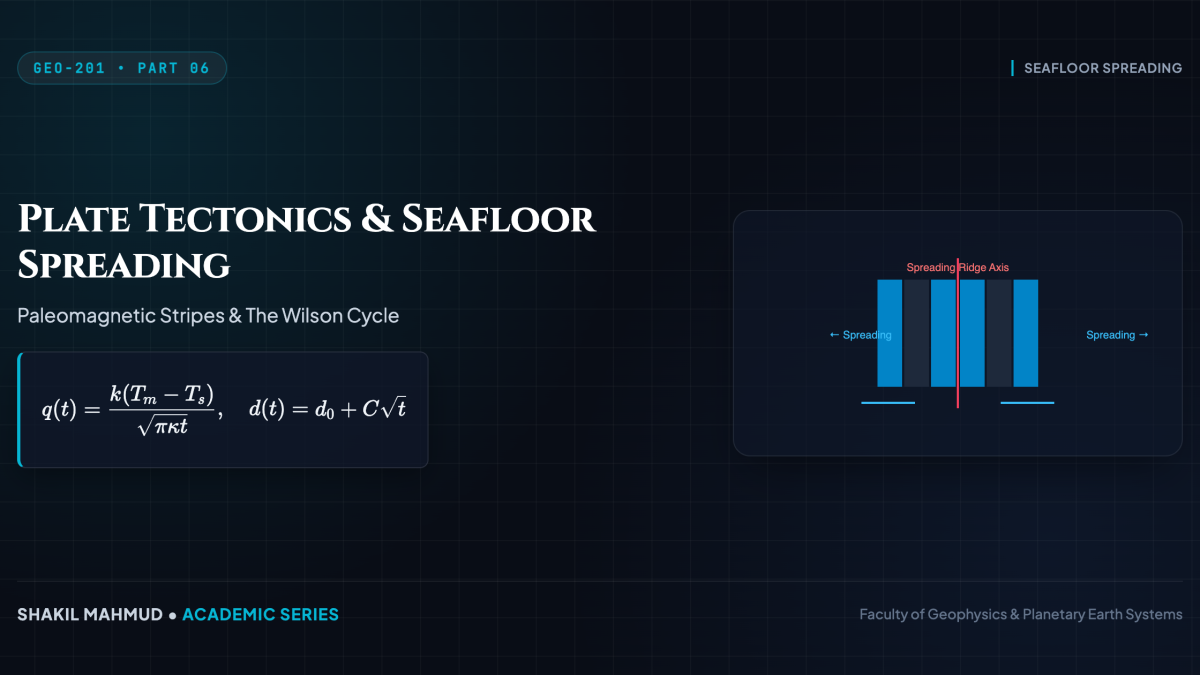
In 1963, Fred Vine, Drummond Matthews, and Lawrence Morley synthesized seafloor spreading with geomagnetic polarity reversals. As basaltic magma ascends at mid-ocean spreading axes and cools below the Curie point ((sim 580^circ ext{C})), ferromagnetic titanomagnetite grains align with Earth’s ambient magnetic vector, acquiring thermoremanent magnetization (TRM).
Because the geomagnetic field periodically reverses polarity, continuous spreading acts as a giant natural tape recorder, creating alternating zebra-striped ribbons of normal and reversed magnetic anomalies symmetrical about the ridge axis. The total magnetic anomaly (Delta B) measured by marine magnetometers is:
[
Delta B = |mathbf{B}_{ ext{obs}}| – |mathbf{B}_{ ext{IGRF}}|
]
Correlating magnetic polarity chron boundaries (e.g., Brunhes, Matuyama, Gauss, Gilbert) with radiometric dates yields precise seafloor spreading rates, ranging from (sim 10 ext{ mm/yr}) on the ultra-slow Gakkel Ridge to (> 160 ext{ mm/yr}) on the ultra-fast East Pacific Rise.
3. Thermal Cooling Model of Oceanic Lithosphere
As newly formed oceanic crust moves away from the spreading axis, it loses heat conductively to the cold ocean water ((T_s approx 0^circ ext{C})). Modeling the lithosphere as a semi-infinite half-space cooling from an initial mantle temperature (T_m approx 1350^circ ext{C}), the one-dimensional thermal diffusion equation:
[
rac{partial T}{partial t} = kappa rac{partial^2 T}{partial z^2}
]
admits the classic similarity solution via the Gauss error function:
[
T(z, t) = T_s + (T_m – T_s) operatorname{erf}left( rac{z}{2sqrt{kappa t}}
ight)
]
where (kappa approx 10^{-6} ext{ m}^2/ ext{s}) is thermal diffusivity. This yields two profound observable geophysical scaling laws:
- Surface Conductive Heat Flow (q(t)): Decays inversely with the square root of seafloor age:
[
q(t) = -k left.rac{partial T}{partial z}
ight|_{z=0} = rac{k(T_m – T_s)}{sqrt{pi kappa t}} propto t^{-1/2}
] - Oceanic Bathymetry Depth (d(t)): Due to thermal contraction, density increases as (
ho(T) =
ho_m [1 – alpha (T – T_m)]). Isostatic subsidence deepens the seafloor proportional to (sqrt{t}):
[
d(t) = d_0 + rac{2
ho_m alpha (T_m – T_s)}{
ho_m –
ho_w} sqrt{rac{kappa t}{pi}} = d_0 + C_b sqrt{t}
]
where (d_0 approx 2500 ext{ m}) at the ridge crest and (C_b approx 350 ext{ m}cdot ext{Myr}^{-1/2}), holding remarkably accurate for seafloor ages (t < 80 ext{ Ma}).
4. The Wilson Supercontinent Cycle
Formulated by J. Tuzo Wilson in 1966, the Wilson Cycle describes the cyclical 400-to-600-million-year lifespan of oceans and supercontinents through six distinct evolutionary stages:
- Embryonic Stage (Continental Rifting): Thermal upwelling thins continental crust, creating grabens and rift valleys (e.g., East African Rift).
- Juvenile Stage (Narrow Seaway): Continued divergence allows seawater incursion and early seafloor spreading (e.g., Red Sea).
- Mature Stage (Wide Ocean Basin): Extensive seafloor spreading forms stable passive continental margins (e.g., Atlantic Ocean).
- Declining Stage (Subduction Initiation): Old, cold oceanic crust collapses under its own negative buoyancy, initiating subduction zones and volcanic arcs (e.g., Pacific Ocean).
- Terminal Stage (Ocean Basin Closure): Narrowing seas and island arc collisions squeeze marine basins (e.g., Mediterranean Sea).
- Suturing Stage (Continental Collision / Supercontinent Assembly): Continent-continent collision closes the ocean entirely, forging major mountain belts and assembling a supercontinent (e.g., Himalayas; Rodinia at (sim 1.1 ext{ Ga}), Pangaea at (sim 300 ext{ Ma})).