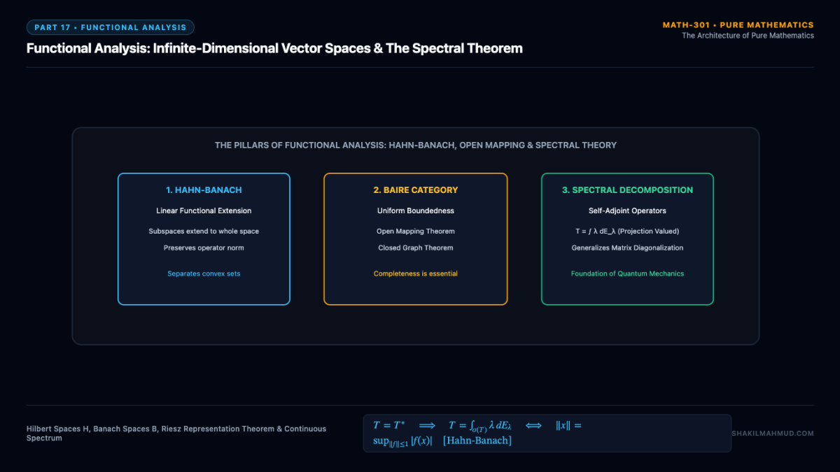
In finite dimensions, all norms are topologically equivalent, unit balls are compact, and linear operators can always be represented by matrices. In infinite dimensions, however, these comfortable intuitions completely shatter. Functional Analysis arose in the early 20th century through the work of David Hilbert, Stefan Banach, and John von Neumann to systematically analyze vector spaces of functions. By fusing linear algebra with metric topology, functional analysis provides the rigorous mathematical language of quantum mechanics and partial differential equations.
1. Banach Spaces & Complete Normed Linear Spaces
A normed vector space $(V, |cdot|)$ is a Banach Space if it is metric complete: every Cauchy sequence ${x_n} subset V$ converges to a limit $x in V$ under the metric $d(x, y) = |x – y|$.
Classical examples include the $L^p(Omega)$ function spaces (equipped with $|f|_p = (int |f|^p dmu)^{1/p}$) and sequence spaces $ell^p$. The geometric anatomy of Banach spaces is governed by the “Three Pillars of Functional Analysis”:
- The Hahn-Banach Theorem: Any bounded linear functional defined on a subspace can be extended to the entire space without increasing its operator norm, guaranteeing a rich dual space $V^*$.
- The Banach-Steinhaus Theorem (Uniform Boundedness Principle): A family of pointwise bounded continuous linear operators is uniformly bounded on bounded sets.
- The Open Mapping & Closed Graph Theorems: Any surjective continuous linear operator between Banach spaces is an open mapping.
2. Hilbert Spaces & The Riesz Representation Theorem
A Hilbert Space $mathcal{H}$ is a Banach space whose norm arises from an inner product: $|x| = sqrt{langle x, x rangle}$. It satisfies the Parallelogram Law:
|x + y|^2 + |x – y|^2 = 2|x|^2 + 2|y|^2
Hilbert spaces possess a notion of orthogonality. Any closed subspace $M subset mathcal{H}$ permits an orthogonal direct sum decomposition: $mathcal{H} = M oplus M^perp$.
By the Riesz Representation Theorem, the continuous dual space $mathcal{H}^*$ is isometrically anti-isomorphic to $mathcal{H}$ itself: for every continuous linear functional $phi in mathcal{H}^*$, there exists a unique vector $y_phi in mathcal{H}$ such that:
phi(x) = langle x, y_phi rangle quad forall x in mathcal{H}
This theorem legitimizes Dirac’s bra-ket notation ($langle phi | x rangle$) in quantum mechanics.
3. Operators: Compact, Self-Adjoint, and Unbounded
A linear operator $T: mathcal{H} to mathcal{H}$ is compact if it maps bounded sets into precompact sets (sets with compact closure). Compact operators are the infinite-dimensional limit of finite-rank matrices.
In quantum mechanics, physical observables (such as position $hat{x} psi(x) = x psi(x)$ and momentum $hat{p} psi(x) = -ihbar frac{dpsi}{dx}$) are represented by unbounded operators defined only on a dense domain $D(T) subset mathcal{H}$. An operator $T$ is self-adjoint if $T = T^*$ and their domains coincide ($D(T) = D(T^*)$).
4. The Spectral Theorem for Self-Adjoint Operators
For an unbounded self-adjoint operator $T$, the spectrum $sigma(T) subset mathbb{R}$ may contain both discrete eigenvalues and a continuous spectrum. The Spectral Theorem states that every self-adjoint operator is unitarily equivalent to a multiplication operator on an $L^2$-space.
In projection-valued measure (PVM) notation, $T$ decomposes into an operator-valued integral over its real spectrum:
T = int_{sigma(T)} lambda , dE(lambda)
This spectral resolution allows one to define functions of operators $f(T) = int f(lambda) dE(lambda)$, yielding the mathematical foundation for quantum time-evolution operators $U(t) = e^{-iHt/hbar}$ and the functional calculus of differential operators.